PROBLEMS

4.1. The two-phase ac servomotor of Problem 3.16 is used in a simple positioning system, as shown in Figure P4.1. Assume that a difference amplifier, whose gain is 10, is used as the error detector and also supplies power to the control field.

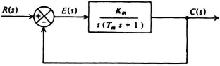
Figure P4.1

(a)  What are the undamped natural frequency ω_n and the damping ratio ζ ?

(b)  what are the percent overshoot and time to peak resulting from the application of a unit step input?

(c)  Plot the error as a function of time on the application of a unit step input.

4.2. Repeat Problem 4.1 with the gain of the difference amplifier increased to 20. What conclusions can you draw from your result?

4.3. The two phase ac servomotor and load, in conjunction with the gear train specified in Problem 3.19, is used in a simple positioning system as shown in Figure P4.1. Assume that a difference amplifier, whose gain is 20, is used as the error detector and also supplies power to the control field.

(a)  What are the undamped natural frequency and damping ratio ζ?

(b)  What are the percent overshoot and time to peak resulting from the application of a unit step input?

(c)  Plot the error as a function of time on the application of a unit step input.

4.4. Repeat Problem 4.3 with the gain of the difference amplifier increased to 40. What conclusions can you draw from your results?

4.5. Repeat Problem 4.3 with the gain of the difference amplifier decreased to 10. What conclusions can you draw from your result?

4.6. A typical aerodynamically controlled missile control system is synthesized by means of the appropriate application of moments to the airframe. These moments are generated by the deflection of control surfaces placed at large distances from the center of gravity. The result is that large moments are created with relatively small surface loads. The design of this type of control system requires a sufficiently high control loop gain in order to minimize the response time to input commands. In addition, it must not be so high as to cause high-frequency instabilities. Figure P4.6 illustrates an acceleration-control steering system of a missile. The command acceleration is compared with the output of an accelerometer to develop the basic error signal which drives the control system. The output of a rate gyro is utilized for damping [3].

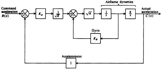
Figure P4.6

(a)  Determine the transfer function C(s)/R(s) of this system.

(b)  Determine the undamped natural frequency ω_n of this system and the damping ratio ζ for the following set of parameters:

amplifier gain = K_a = 16,   aircraft gain factor = q = 4,   K_R = 4.

(c)  Determine the percent overshoot and time to peak resulting from an input command of a unit step of acceleration.

4.7. Figure P4.7 illustrates the control system of a map drive system used to display a portion of the map of an area to the commander of a task force. A main requirement of this control system is that a constant tension be maintained on the continuous sheet of paper between the wind-up and wind-off rolls in order that the paper does not tear. The system illustrated contains four rollers, and a spring which provices a restoring angular torque of K₁θ(t). As the radius R of the rollers varies, the tension changes and an adjustment in the wind-up motor speed is required. The map leaving the wind-off roll is assumed to have a velocity v₁(t) and a tension T₂(t); that approaching the wind-up roll is assumed to have a velocity v₂(t) and a tension T₁(t). A synchro-type sensing device, whose transfer function is K_e, is mounted on the pivot point of the tension arm and is used to sense angular deviations from θ = 0. This error signal is amplified by a factor K_a by an amplifier. In addition, assume that the relationship for motor control voltage E_c(t) caused by tension variations T(t) is given by

E_c(t) = K₂T(t).

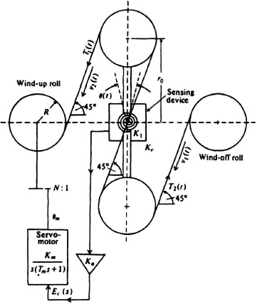
Figure P4.7

The two-phase ac servomotor is assumed to have a transfer function given by Eq. (3.101). It also contains a gear reduction of N : 1.

(a)  Determine the transfer function relating the change in tension T(s) due to an input change velocity v₁(s) of the wind-off roll in terms of the system parameters.

(b)  Determine the undamped natural frequency ω_n and the damping ratio ζ in terms of the system parameters.

(c)  Calculate the damping ratio ζ for the case of a fully loaded wind-up roll, with the following parameters:

inertia of wind-up roller	= 0.101 oz in sec2,
gear ratio	= N = 10.4 : 1
radius of wind-up roller	= R = 1.5 in,
motor inertia	= Jm = 4.43 × 10−4 oz in sec2,
motor constant	= Km = 0.417 in oz/(rad/sec),
synchro sensitivity	= Ke = 0.4 V/degree,
amplifier gain	= Ka = 1000,
K1	= 10.5 V/oz/tension,
K2	= 0.04 in oz/degree.

(d)  How can the damping ratio be increased?

4.8. The Viking Mission conducted by the National Aeronautics and Space Administration included two launches in 1975 of a Viking Spacecraft by a Titan-Centaur launch vehicle consisting of an Orbiter and a Lander. The Orbiter had the capability of orbiting the planet Mars and of separating the Lander capsule, an automated laboratory in the search of signs of life, that entered the Martian atmosphere for soft landing on the surface of Mars. Looking over Mars from orbit, Viking cameras and other instruments aided in the confirmation of a suitable landing site. After this confirmation, the Lander separated from the Orbiter and began its descent to the Martian surface. The descent occurred when Mars was about 225 million miles from Earth and nearly on the other side of the Sun. Therefore, this required a completely automated deorbit and landing operation because two-way communication at that distance was almost 45 minutes. Viking featured a series of scientific experiments in the areas of biology, geology, and meteorology. In order to collect material for these experiments, the Lander had a retractable claw with a 10-ft reach, as shown in Figure P4.8a. It was used for scooping out soil samples and placing them in its automated chemical laboratory for analysis. For purposes of this example, assume that the control system which positions the retractable claw can be represented by the second-order control system shown in Figure P4.8b.

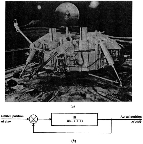
Figure P4.8   (a) Lander capsule, Viking Project. (Official NASA photo) (b) Block diagram of the second-order control system for positioning the retractable claw.

(a)  Determine the undamped natural frequency and the damping ratio of this control system.

(b)  Determine the maximum percent overshoot and time to peak resulting from the application of a unit command signal.

4.9. A two-phase ac induction motor is used to position a device in a feedback configuration represented by Figure P4.1. The time constant of the motor and load, T_m, is 0.5 sec.

(a)  Determine the combined amplifier and motor constant gain K_m which will result in a damping ratio of 0.5.

(b)  What is the resulting undamped natural frequency for the value of gain determined in part (a)?

4.10. A simulator used for training the crew of an aircraft is to be designed. The simulator will have a two-degree-of-freedom capability (roll and pitch), which will give the trainees a feel of the dynamics which the aircraft crew will experience during operating conditions. A typical aircraft trainer of this type is usually driven by a digital computer which provides the control inputs/logic of the system. The controls and interior of the simulator will be designed to be a very close replica of the actual aircraft, and give the trainees a real-world feel of the aircraft—both esthetically and dynamically. For purposes of this analysis, assume that the pitch loop can be represented by Figure P4.10.

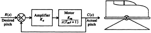
Figure P4.10

Test data of the aircraft dynamics show that pitch can closely be approximated by a critically damped loop. Assuming that ζ = 1, K_m = 5 and T_m = 1, determine the following:

(a)  The resulting undamped natural frequency of the system, ω_n.

(b)  Amplifier gain K_a required to achieve critical damping.

4.11. Robotics have revolutionized the manufacturing industry, and this is especially true in the manufacture of automobiles. Figure P4.11a shows a photograph of the GMFanuc Robotics Corporation Model P-150 six-axis (a seventh axis is optional) articulated arm, electric-servo-driven robot painting an automobile. All axis motions are controlled simultaneously [4]. All axes are driven by state-of-the-art compact ac servomotors providing fast acceleration and deceleration, precision painting, and no brush maintenance.

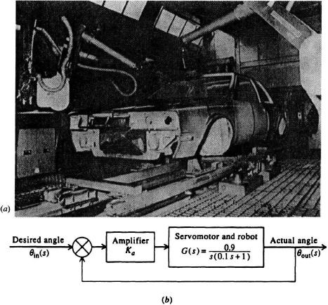
Figure P4.11   (a) Photograph of the GMFanuc Robotics Corporation Model P-150 six-axis (a seventh axis is optional) articulated arm, electric-servo-driven robot painting an automobile. (Courtesy of GMFanuc Robotics Corporation) (b) Block diagram.

Let us assume that we have to design a robot such as this one, and that one of the axes can be represented by the block diagram shown in Figure P4.11b. For the purposes of our application, a critically damped system will be assumed to be desirable. Find the amplifier gain K_a that will achieve a critically damped system.

4.12. It is desired to analyze the response of the feedback configuration shown in Figure P4.12 used to position a device in response to an input. The motor selected for this application has a motor constant K_m = 0.4 and a motor time constant T_m = 0.1. For an amplifier gain K_a = 20, determine the following:

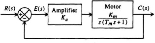
Figure P4.12

(a)  What is the undamped natural frequency ω_n?

(b)  What is the damping ratio ζ ?

(c)  Determine the maximum percent overshoot resulting from the application of a unit step input?

(d)  Find the time to peak, t_p, for the unit step input applied in part (c).

(e)  Sketch the output c(t) and error e(t) resulting from the application of a unit step input r(t). Indicate the time to peak and the maximum overshoot on your sketch.

4.13. For Figure P4.13 determine the following:

(a)  Undamped natural frequency, ω_n.

(b)  Damping ratio ζ.

(c)  Maximum percent overshoot.

(d)  Time to peak, t_p.

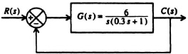
Figure P4.13

4.14. Repeat Problem 4.13 for

4.15. A robot is used on an airplane assembly line to drill some holes. The block diagram of the control system used to control the drill in one axis is shown in Figure P4.15.

Figure P4.15

(a)  Determine the amplifier gain K_a required to achieve a damping ratio in the system of 0.7.

(b)  Calculate the corresponding time to peak.

(c)  Calculate the corresponding maximum percent overshoot.

4.16. A control-system engineer needs to use a two-phase ac servomotor for an application on a project which is running short of money. The stock room has a spare motor, but the name plate is missing. The control-system engineer needs to determine the motor constant, K_m, and the motor time constant, T_m, before this motor can be used in the application. To accomplish this, the engineer hooks up the simple positioning control system shown in Figure P4.16a containing this two-phase ac servomotor and applies a unit step input.

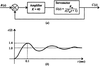
Figure P4.16

The response of this control system to a unit step is illustrated in Figure P4.16b.

From this response, determine, K_m and T_m.

4.17. The exact transfer function of a second-order system is unknown. We wish to determine its transfer function by applying a unit step to its input, r(t), and analyzing its output response, c(t), shown in Figure P4.17.

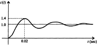
Figure P4.17

Determine it transfer function, C(s)/R(s).

4.18. A robot is used to drill holes in the body of an automobile on an assembly line in response to commands as in Figure P4.18. For this application, a critically damped system is desired.

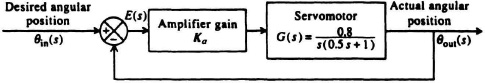
Figure P4.18

(a)  Determine the amplifier gain K_a required to achieve a critically damped system.

(b)  Sketch r(t), c(t), and e(t) on the same set of axes when r(t) is a unit step input.

(c)  Determine the time t when the error e(t) and the output c(t) are equal.

4.19. We wish to fit the data contained in Table P4.19 to a model. These data represent the transient response of the following closed-loop transfer function to a unit step input:

We wish to fit this data with the following model:

c(t) = 1 + K₁e^−at + K₂e^−bt

(a)  Focus only on the slowest or smallest root, and determine

K₁e^−at

by subtracting the steady-state value of one from the data, and fitting a straight line to the log₁₀ of the difference. Determine K₁ and a.

(b)  Plot the log₁₀ of c(t) − c_ss − K₁e^−at, and determine K₂ and b from the resulting straight line.

(c)  Having determined K₁, K₂, a, and b, determine the estimated value of ĉ(t).

(d)  Compare the resulting estimated value of ĉ(t) with the theoretical value of c(t) provided in Table P4.19.

(e)  Plot the theoretical and graphical values of the theoretical value of c(t) with the estimated value of ĉ(t) on the same set of axes. In addition, plot the error between the two sets of data on this same set of axes.

(f)  How well does your fit of ĉ(t) compare with the theoretical value of c(t)?

(g)  Determine the modeled value of Ĉ(s)/R(s).

Table P4.19. Set of data representing the theoretical value of c(t).

Time	c(t)
0	0
0.2000	0.1735
0.4000	0.4145
0.6000	0.6012
0.8000	0.7314
1.0000	0.8197
1.2000	0.8791
1.4000	0.9189
1.6000	0.9457
1.8000	0.9636
2.0000	0.9756
2.2000	0.9836
2.4000	0.9890
2.6000	0.9926
2.8000	0.9951
3.0000	0.9967
3.2000	0.9978
3.4000	0.9985
3.6000	0.9990
3.8000	0.9993
4.0000	0.9996
4.2000	0.9997
4.4000	0.9998
4.6000	0.9999
4.8000	0.9999
5.0000	0.9999