
6.17. ROOT-LOCUS METHOD FOR CONTROL SYSTEMS USING MATLAB [7]
In Sections 6.14–6.16, several root-locus plots were generated using the 12 rules of construction and were hand drawn. Additionally, several root-locus plots were also illustrated which were obtained using MATLAB. In this section, the reader will be shown how to obtain the root-locus diagrams very easily and accurately using MATLAB.
A. Drawing the Root Locus if the System is Defined by a Transfer Function
The MATLAB command used for plotting the root locus is
rlocus(num,den)
The Modern Control System Theory and Design (MCSTD) Toolbox enhances the professional toolbox by not only plotting the root locus with “rlocus” but also calculating almost any point of interest on the root-locus plot directly (the professional version has only “rootfind,” a graphical method, to locate these points). The most commonly required value, Kmax, can now be obtained directly using the MCSTD Toolbox.
What is left now is to understand how to create root-locus diagrams, and to practice creating them. There are many examples of creating root-locus diagrams on the MCSTD diskette (try some). Several functions exist that assist with root-locus diagrams, of which I have listed ones that I believe are important:
- “rlocus” is described in Reference 7. This function returns/plots the root-locus response of the system. A single example is given in the text manual.
- “rlaxis” is described in the MCSTD Toolbox. This function returns a set of data representing the portion of the root locus that is on the real axis.
- “rlpoba” is described in the MCSTD Toolbox. This function returns the value(s) (with their associated gains) of the breakaway/break-in points of the root locus.
- “rootmag” is described in the MCSTD Toolbox. This function returns the value(s) (with their associated gains) of any point on the root locus that corresponds to the specified magnitude. In the discrete root locus, a magnitude of 1 corresponds to Kmax.
- “rootangl” is described in the MCSTD Toolbox. This function returns the value(s) (with their associated gains) of any point on the root locus that corresponds to the specified angle. In the continuous root locus, an angle of ±90 corresponds to Kmax. Also, desired gains that accomplish specified damping factors (corresponding to particular angles), can easily be picked off (usually presented in compensation and design using the root locus).
These MCSTD features/utilities alone make the MCSTD Toolbox well worth any design engineer’s review. Most of the critical values that normally have to be picked off the plot can be calculated directly using the MCSTD Toolbox. The Kmax value, indicating the maximum gain before instability occurs, is calculated. Breakaway and break-in points of the root locus are also calculated in the MCSTD Toolbox, instead of by doing them by hand.
When trying to find the proper syntax to call the “rlocus” utility, either use the help feature or look in the reference manual. Valid syntax for the “rlocus” utility is described in Reference 7. Like the Bode utility, the left-hand arguments (r and k) are optional for this function.
Other functions dealing with the root locus are also available only in the MCSTD Toolbox. The MCSTD demo M-file does elaborate further on the creation of the root locus and the important associated points of interest, with on-screen examples. The significance of these utilities will be understood as you progress to the appropriate topics (e.g., discrete time system analysis).
To illustrate the use of MATLAB for obtaining the root locus, let us reconsider the root locus plotted in Figure 6.61b for the negative-feedback control system defined by Eq. (6.166) which is repeated here:
In order to ease its transformation to MATLAB notation, we multiply all terms in the numerator and denominator (or use the MATLAB “conv” command):
Therefore, the row matrices for the numerator and denominator are as follows:
num = [0 0 0 1.6 16]
den = [1 9 24 16 0].
Because the root locus goes to infinity, it can lead to difficulties when using MATLAB. Therefore, we have to limit the area of the root locus drawn in the same manner we did for the Nyquist diagram which was discussed in Section 6.6. Therefore, we also add the command “v = [−14 4 −5 5]; axis (v).” The resulting MATLAB program to draw the root locus is given in Table 6.21.
The resulting root locus diagram obtained using MATLAB is illustrated in Figure 6.68 and Fig. 6.61b.
Table 6.21. MATLAB Program for Obtaining the Root Locus for the System Defined by Eq. (6.189)
| num = [0 0 0 1.6 16] den = [1 9 24 16 0] rlocus(num,den) v = [−14 4 −5 5]; axis(v) title(‘Root Locus of Unity Feedback System where G(s) is given by Eq. (6.189)’) |
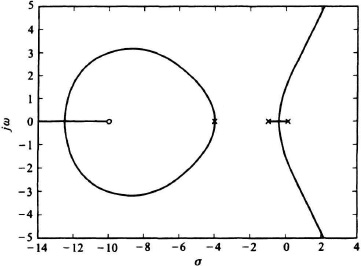
Figure 6.68 Root locus of unity-feedback system where G(s) is given by Eq. (6.189).
The MCSTD Toolbox contains many additional commands which can greatly aid the control-system engineer in finding additional important information on the root locus. These are illustrated as follows:
(a) Determining portions of the real axis which are part of the root locus: Use the command rlaxis(num,den). The program output for this problem is
−∞ − 10.0000
−4.0000 − 4.0000
−1.0000 0
(b) Determining the point of breakaway and or break-in of the root locus, and the value of the gain K at these points: Use the command rlpoba(num,den). The program output for this problem is
kbreak =
2.5964e + 003
0
2.0417e − 001
sbreak =
– 12.4812
– 4.0000
– 0.4435
(c) Determining the gain at the crossing of the imaginary axis, and the imaginary axis value: Use the command rootangl(num,den,angle), and set the angle portion equal to 90 as follows:
rootangl(num,den,90)
The program output for this problem is
kimag =
3.1692
simag =
0.0000 + 1.5301i
The MATLAB Program of Table 6.21 is modified to add and display the additional commands of rlaxis, rlpoba, and rootangl in the MATLAB Program in Table 6.22.
The resulting root locus containing the original root-locus plot shown in Figure 6.68 and the additional information obtained from the three commands rlaxis, rlpoba, and rootangl is shown in Figure 6.69. This problem is also shown in DEMO 4 of the MCSTD Toolbox where additional features for drawing the root locus from commands found in the MCSTD Toolbox are illustrated.
Table 6.22. MATLAB Program of Table 6.21 with Additional Command of rlaxis, rlpoba, and rootangl
| num = [0 0 0 1.6 16] den= [1 9 24 16 0] rlocus(num,den) v = [−14 4 −5 5]; axis(v) realaxis = rlaxis(num, den) [kbreak,sbreak] = rlpoba(num,den) [kimag,simag] = rootangl(num,den,90) disp(‘realaxis = rlaxis(num,den);’) disp(‘[kbreak,sbreak] = rlpoba(num,den);’) disp(‘[kimag,simsag] = rootangl(num,den,90;’) title(‘Root locus of Figure 6.68 with Additional Points of Interest Labeled’) |
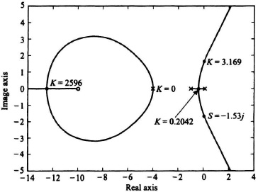
Figure 6.69 Root locus of Figure 6.68 with additional points of interest labeled.
B. Drawing the Root Locus if the System is Defined in State-Space Form
The MATLAB command for this case is given by
rlocus(A,B,C,D).
As was demonstrated previously in this chapter (e.g., Section 6.6 on the Nyquist Diagram, and Section 6.8 on the Bode diagram), we must first obtain the state-space form and then use this new command.
To demonstrate this procedure, let us obtain the state-space form from the transfer function given by Eq. (6.189) using the MATLAB command
[A,B,C,D] = tf2ss(num,den)
whose application has been demonstrated before with the sections on the Nyquist diagram (Section 6.6) and the Bode diagram (Section 6.8). The resulting MATLAB program for accomplishing this is shown in the MATLAB program in Table 6.23.
Therefore, the resulting MATLAB program for obtaining the root locus of this problem from the state-space formulation is given by the MATLAB program in Table 6.24. The resulting root locus diagram is identical to that shown in Figure 6.68.
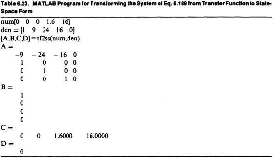
Table 6.24. MATLAB Program for Obtaining the Root Locus for the System Defined by Eq. 6.169 from its State-Space Form determined in Table 6.23
| A = [−9 −24 −16 0; 1 0 0 0; 0 1 0 0; 0 0 1 0]; B = [1; 0; 0; 0]; C = [0 0 1.6 16]; D = [0]; rlocus(A,B,C,D) v = [−14 4 −5 5]; axis(v) title(‘Root Locus of Unity Feedback System where G(s) is given by Eq. (6.188)’ |