6.14.  ROOT-LOCUS METHOD FOR NEGATIVE-FEEDBACK SYSTEMS

The root-locus method is a technique for determining the roots of the closed-loop characteristic equation of a system as a function of the static gain. This method is based on the relationship that exists between the roots of the closed-loop transfer function and the poles and zeros of the open-loop transfer function. The root-locus method, which was conceived by Evans [23, 25], has several distinct advantages.

Knowledge of the location of the closed-loop roots permits the very accurate determination of a control system’s relative stability and transient performance. Alternatively, approximate solutions may be obtained, with a considerable reduction of labor, if very accurate solutons are not required. This and the following section present the graphical method of constructing the root locus and of interpreting the results for negative- and postive-feedback systems, respectively. Working digital computer programs for obtaining the root locus are presented in Section 6.17 (using MATLAB) and 6.18. The technique for synthesizing a system utilizing the root-locus method is discussed in Section 7.9. The method is a useful one and should be part of the designer’s bag of tricks.

Let us consider the general feedback control system illustrated in Figure 6.55. In order to find the poles of the closed-loop transfer function, we require that

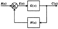
Figure 6.55   A nonunity-feedback control system.

where n = 0, ±1, ±2, ... Equation (6.131) specifies two conditions that must be satisfied for the existence of a closed-loop pole.

1. The angle of G(s)H(s) must be an odd multiple of π:

   

   
   where n = 0, ±1, ±2, ...
2. The magnitude of G(s)H(s) must be unity:

The construction of the root locus for a particular system can start by locating the open-loop poles and zeros in the complex plane. Other points on the locus can be obtained by choosing various test points and determining whether they satisfy Eq. (6.132). The angle of G(s)H(s) can be easily determined at any test point in the complex plane by measuring the angles contributed to it by the various poles and zeros. For example, consider a feedback control system where

At some exploratory point s_E, G(s)H(s) has the value

Graphically, Eq. (6.135) can be represented by Figure 6.56 where the vectors

α = s_E + s_A,

β = s_E + s_B,

γ = s_E + s_C,

δ = s_E + s_D,

= s_E.

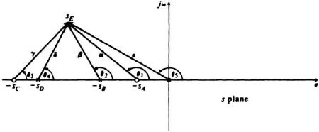
Figure 6.56    Vector representation of at the exploratory point s_E.

The angle of G(s_E)H(s_E) is the sum of the angles θ₁, θ₂, θ₃, θ₄, and θ₅, determined by the vectors α, β, γ, δ, and , respectively:

If this angle equals (2n + 1)π where n = 0, ±1, ..., then s_E lies on the root locus. If it does not, the point s_E does not lie on the locus and a new point must be tried. When a point is found which does satisfy Eq. (6.132), the vector magnitudes are determined and are substituted into Eq. (6.133) in order to find the value of the gain constant K at the exploratory point s_E:

Fortunately, the actual construction of a root locus does not entail an infinite search through the complex plane. Because the zeros of the characteristic equation are continuous functions of the coefficients, the root locus is a continuous curve. Therefore, the root locus must have certain general patterns that are governed by the location and number of open-loop zeros and poles. Once these governing rules are established, the drawing of a root locus is not a tedious and lengthy trial-and-error procedure. We next present 12 basic rules that aid in determining the approximate location of the root locus.

Rule 1. The number of branches of the locus equals the order of the characteristic equation. This is because there are as many roots (and branches) of the root locus as the order of the characteristic equation. Each segment, or branch, of the root locus describes the motion of a particular pole of the closed-loop system as the gain is varied.

Rule 2. The open-loop poles define the start of the root locus (K = 0), and the open-loop zeros define the termination of the root locus (K = ∞). This can easily be shown by considering Eq. (6.137). At open-loop zeros, K must approach infinity because there is a zero in the numerator due to either s_A or s_C and the expression equals 1. However, K must approach zero when open-loop poles occur because there is a zero in the denominator due to the pole at the origin, s_B or s_D and the expression equals 1. When the order of the denominator of G(s)H(s) is greater than the numerator, the root locus ends at infinity, whereas if the order of the numerator is greater than the denominator, the root locus starts at infinity.

This can be illustrated by considering the following characteristic equation of the control system:

Rearranging Eq. (6.138), the following is obtained:

To demonstrate that the points on the root locus which correspond to K = 0 are open-loop poles, let us let K approach zero in Eq. (6.139) as follows:

Therefore, as K approaches zero, a pole must exist (s must approach one of the open-loop poles). Therefore, each branch of the root locus must start at a pole of the open-loop transfer function, G(s)H(s). Now let us consider what happens as K is increased to infinity. For this case, each branch of the root locus approaches either a zero of the open-loop transfer function, G(s)H(s), or infinity in the complex plane. To demonstrate that the points on the root locus which correspond to K equals to infinity are open-loop zeros, let K approach infinity in Eq. (6.139) as follows:

Therefore, as K approaches infinity, a zero must exist (s must approach one of the open-loop zeros). Note that there are the same number of poles and zeros in a root locus, if we include the zeros at infinity in the count. This is at it should be since every branch of the root locus starts at a pole (K = 0) and ends (terminates) at a zero (K = ∞).

Rule 3. Complex portions of the root locus always occur as complex-conjugate pairs if the characteristic equation is a rational function of s having real coefficients. Therefore, the root locus for this condition is symmetrical with respect to the real axis.

Rule 4. Sections of the real axis are part of the root locus if the number of poles and zeros to the right of an exploratory point along the real axis is odd. This is easily demonstrated from Eq. (6.132). Because the angular contribution along the real axis due to complex-conjugate poles cancels, the total angle of G(s)H(s) is due only to the contributions of the real poles and zeros. Therefore, at any exploratory point along the real axis, the angular contribution due to a pole or zero to its right is 180°, whereas that due to a pole or zero to its left is zero.

Rule 5. Angles of asymptotes to the root locus α_m are given by [25]

where

p = number of finite open-loop poles,

z = number of finite open-loop zeros,

m = 0, 1, 2, ..., up to m = p − z (exclusively).

Although m can have an infinite number of values as m is increased, the angle α_m repeats itself, and the number of distinct asymptotes is p − z.

To determine the asymptotes of the root locus, consider a test point s_E which is located very far from the origin. For this condition, the angle of each complex quantity can be considered to be the same. Open-loop poles then cancel the effect of open-loop zeros. Therefore, the root loci for very large values of s are asymptotic to straight lines. Because the total angular component must add up to ±180° or some odd multiple, Eq. (6.142) follows. Figure 6.57 illustrates the asymptotes of a third-order system where

The asymptotic angles for the root locus illustrated in Figure 6.57 are

α₀ = ±π/3 = ±60°     
α₁ = ±3π/3 = ±180°.

Rule 6. The intersection of the asymptotes and the real axis occurs along the real axis at s_r, where [25]

The value of s_r is the centroid of the open-loop pole and zero configuration.

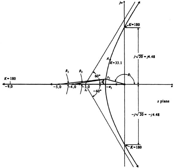
Figure 6.57   Root locus of a system where .

To determine the intersection of the asymptotes and the real axis, let us expand the numerator and denominator of the following open-loop transfer function:

We are interested in a test point which is located very far from the origin of the s-plane. For this case, Eq. (6.145) can be rewritten as follows:

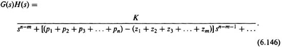
Substituting Eq. (6.146) into the characteristic equation

we obtain the following result:

For very large values of s, Eq. (6.144) can be approximated as follows:

Let us denote the intersection of the asymptotes and the root locus by s_r. Therefore,

Note that s_r is always a real number because complex zeros and poles always occur in complex-conjugate pairs.

The intersection of the asymptotes for the root locus illustrated in Figure 6.57 is given by

Rule 7. Consider the simple case where the locus has a branch on the real axis between two poles as shown in Figure 6.58a. A point must exist where the two branches break away from the real axis and enter the complex region of the s-plane in order to approach zeros which are finite or are located at infinity. Because K has a value of zero at the two poles and increases in value as the locus moves along the real axis away from the poles, the K’s for the two branches simultaneously reach a maximum value at the breakaway point. A plot of |K| versus σ is shown in Figure 6.58b. For the case where the locus has branches on the real axis between the two zeros as illustrated in Figure 6.58c, branches come from poles in the complex region and break in onto the real axis. The variation in value of |K| along the real axis locus between these two zeros is shown in Figure 6.58d. The two poles that enter the real axis and then move to zeros on the real axis will enter simultaneously with a value of K, which is a minimum because the gain is increasing continuously as the loci approach the zeros. Thus the breakaway and break-in-points can be evaluated from the magnitude condition for Re s = σ and solving for K(σ). This can be accomplished graphically or by solving

Figure 6.58   Loci for two consecutive poles and zeros on the real axis and the corresponding relation of |K| versus s.

to find all the maxima and minima of K(σ) and their locations. The most straight-forward method for isolating the factor K is to rearrange the characteristic equation. An example will illustrate the procedure.

For the system analyzed in Figure 6.57

The characteristic equation of this system is given by

Alternatively, this can be written as

K = −s(s + 4)(s + 5).

For the case of Re s = σ, we obtain

K(σ) = −σ(σ + 4)(σ + 5).

Multiplying the factors together, we have

K(σ) = −σ³ − 9σ² − 20σ.

Taking the derivative of this function and setting it equal to zero, we can determine the breakaway point:

The roots are

σ₁ = −1.47,
σ₂ = −4.53.

The breakway point of σ₁ is indicated in Figure 6.57; the value of σ₂ is not a possible solution in this negative-feedback example because the root locus does not exist on the real axis at this point. It is interesting to note that the point −4.53 is a breakaway point for this system when there is positive feedback present (see Section 6.16).

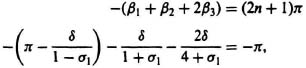
Points of breakaway of the root locus from the real axis can also be obtained by considering the transition from the real axis to a point s₁, which is a small distance δ off the axis. The basis of this method is that the transition from the real axis to s₁ must result in a zero net change of the angle of G(s)H(s). This is illustrated for the root locus considered in Figure 6.57. For this example,

The very small angles we are considering are equal to their tangents, in radians, as follows:

This can be rewritten as

Canceling δ, and simplifying, results in the equation

Solution of Eq. (6.153) yields the absolute values of σ₁ equal to −1.47 and −4.53. As indicated before, the value of −4.53 is impossible for negative feedback.

Both techniques presented for determining the breakaway and break-in points are utilized in this book. They are referred to as the maximization (or minimization) of K(σ) and the transition methods.

Rule 8. The intersection of the root locus and the imaginary axis can be determined by applying the Routh–Hurwitz stability criterion to the characteristic equation. The characteristic equation for the system illustrated in Figure 6.57 is given by

The resulting Routh–Hurwitz array is given by

For this simple array, a zero in the third row indicates a pair of complex-conjugate poles crossing the imaginary axis. The corresponding maximum value of gain and the value of s at which this occurs can be obtained as follows: For the third row to equal zero,

or

Therefore, this system is stable for all gains up to a value of 180. The corresponding value of s occurring at the crossing of the imaginary axis can be obtained from the characteristic equation, Eq. (6.154), with K = 180 and s = jω. We can either set the real part of Eq. (6.154) equal to zero, or we can set the imaginary part of Eq. (6.153) equal to zero. Either approach will give us the correct value for the crossing of the imaginary axis. Using the real parts, we find that

–9ω² + 180 = 0,

or

These values are illustrated in Figure 6.57.

Rule 9. The angles made by the root locus leaving (or entering) a complex pole can be evaluated by applying the principle of Eq. (6.132). This is illustrated by considering the system shown in Figure 6.59. As indicated in Figure 6.59, Rule 5 shows that the asymptotes are at ±60°, and Rule 6 shows that the intersection of the asymptotes and the real axis is at −1.33. We can find K_max and the crossing of the imaginary axis from Rule 8 as follows. The characteristic equation for the system shown in Figure 6.59 is given by

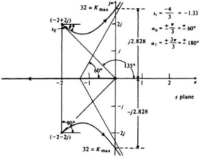
Figure 6.59   Root locus of system where .

Therefore, its Routh–Hurwitz array is given by

Setting U₁ = 0, we find that K_max = 32. The crossing of the imaginary axis can be found by setting the real or imaginary terms of Eq. (6.157) equal to zero with K = 32. Using the real terms,

Therefore, we find that the root locus crosses the imaginary axis at s = ±j2.828 as shown in Figure 6.59.

Let us calculate the angle that the root locus makes with the complex pole located at −2 + 2j. An exploratory point s_E will be assumed slightly displaced from this pole. The angle made by the root locus leaving the pole at −2 + 2j to the point s_E is assumed to be −θ, as illustrated in Figure 6.59. This angle is defined as the angle of departure. The angles contributed to the point s_E, due to various open-loop poles of the system, must conform with Eq. (6.132) and are given by (see Figure 6.59)

–135° − 90° + θ = −180°,
                    θ = 45°.

Therefore, the angle contributed by the branch of the root locus leaving the pole at −2 + 2j must be sufficient to satisfy the basic relationshp given by Eq. (6.132). The negative sign appears before aech of the angles in this angular equation, because they are in the denominator of the expression given by Eq. (6.132). If zeros were present, however, they would contribute positive angles, because they are in the numerator of the expression given by Eq. (6.132). If we had assumed θ to be in the wrong direction, then our answer for θ would be negative.

Rule 10. In order to derive a useful relation between the poles of the open-loop transfer function and the roots of the characteristic equation, consider the following form of the open-loop transfer function for the system illustrated in Figure 6.55, where z_i represents the open-loop zeros and p_a represents the open-loop poles excluding those at the origin:

In practical physical systems

n + y > x,

and the denominator of C(s)/R(s) is of the form

where

m = n + y

r_j = roots described by the root locus.

Substituting Eq. (6.159) into Eq. (6.160) and equating the expressions on each side of the resulting equation, gives the following:

Expanding the product terms of this equation yields

For those open-loop transfer functions where the denominator of G(s)H(s) is at least of degree 2 higher than that of the numerator (which is often the case in practice)

x m − 2,

and the following is obtained by equating the coefficients of s^m−1 in Eq. (6.161):

By defining p_j to represent all of the open-loop poles, incuding those at the origin, this equation can be written as

Equation (6.162), known as Grant’s rule, indicates the sum of the system roots is a constant as the gain is varied from zero to infinity. Therefore, the sum of the system roots is conserved and is independent of gain. This rule, sometimes also referred to as the conservation of the sum of the roots, aids in the drawing the root locus, because it implies that as certain loci turn to the right, others must turn to the left in order that the sum of the closed-loop poles may be constant. In addition, this rule, as described by Eq. (6.162), aids in determining the gain along the root locus. For interest, we can determine the location of the third root of the system illustrated in Figure 6.57 when the root locus crosses the imaginary axis as follows:

Therefore, at r = −9, the gain is also 180.

Rule 11. The gain along the root locus can be determined in a number of ways. One of the two fundamental rules of the root locus, Eq. (6.133), can be used to determine this as indicated previously in Figure 6.56 and Eq. (6.137). Basically, for any point along the root locus, the control-system engineer can substitute the distance of the various poles and zeros to the point into Eq (6.133) and solve for K. As an example, let us reconsider the root locus illustrated in Figure 6.57. We have already determined that the gain when the root locus intersects the imaginary axis is 180 (using rule 8). Now, let us determine the value of gain at point A. To do this, we need to solve the following equation:

Measuring the distances |s_A|, |s_A + 4|, and |s_A + 5| to be 2.2, 3.5, and 4.3, respectively, and substituting these values into Eq. (6.163), we obtain

Gains along the rest of the root locus can be similarly determined.

Rule 12. The root locus never crosses itself. The accuracy of the root locus constructed can be greatly improved by use of the digital computer to implement the rules of construction. In Section 6.17, the application of MATLAB to obtaining the root locus is demonstrated. In Section 6.18, a working program for constructing the root locus is presented for those readers who do not have MATLAB available. Other commercially available software packages for constructing the root locus are presented in Section 6.18. Many of the root-locus plots presented hereafter in this book are constructed using either this digital computer program, or the MATLAB program.

This section will conclude with illustrative examples of the root-locus procedure. The techniques of stabilizing systems utilizing the root-locus method are illustrated also in Chapters 7, 8, 9 and 12.

Example 1

As the first example, consider a unity negative-feedback system whose open-loop transfer function is given by

This system has four poles: three on the negative real axis and one on the positive real axis. In addition, it has four zeros at infinity. The root locus of this system, illustrated in Figure 6.60, can be drawn on the basis of the 12 rules, as follows.

Rule 1. There are four separate loci, as the characteristic equation, 1 + G(s)H(s), is a fourth-order equation.

Rule 2. The root locus starts (K = 0) from the poles located at 1, −1, and a double pole at −4. All loci terminate (K = ∞) at zeros, which are located at infinity for this problem.

Rule 3. Complex portions of the root locus occur in complex-conjugate pairs, and the root locus is symmetrical with respect to the real axis.

Rule 4. The portions of the real axis between −1 and 1, and the point −4 are part of the root locus.

Figure 6.60   Root locus of system where .

Rule 5. The four loci approach infinity as K becomes large at angles given by

α₀ = ±π/4 = ±45°

and

α₁ = ±3π/4 = ±135°.

Rule 6. The intersections of the asymptotic lines and real axis occur at

Rule 7. The point of breakaway from the real axis is determined using the two techniques presented: maximization of K(σ) and the transition methods.

Maximization of K(σ) Method. From the equation

we obtain

The roots are

σ₁ = 0.22,    σ₂ = −2.22,    σ₃ = −4.

Of these, σ₁ represents the breakaway point from the positive real axis, and σ₃ represents the breakaway from the double pole at −4, 0 for this negative feedback system. The value of σ₂ represents the breakaway point for positive feedback (see Problem 6.48).

Transition Method. The point of a breakaway from the real axis occurring between −1 and 1 will be assumed to lie along the positive real axis at σ₁. The angles contributed from the various poles to a point s₁ that lies a small distance δ off the positive real axis are

or

Solving, we obtain roots at 0.22, −2.22 and −4. The interpretation of these roots is the same as with the first method.

Rule 8. This particular root locus intersects the imaginary axis only at the origin.

Rule 9. This rule does not apply to this problem.

Rule 10. This rule shows that as certain of the loci turn to the right, others turn to the left to ensure that the sum of the roots is a constant.

Rule 11. This rule does not apply to this problem, because the problem does not require the calculation of gains along the locus.

Rule 12. The root locus does not cross itself.

It is interesting to observe from the root locus illustrated in Figure 6.60 that the system is always unstable because at least one root of the characteristic equation always lies in the right half-plane. We illustrate in Section 7.9 the stabilization of this system by means of a lead network, and by using a minor loop containing rate feedback.

Example 2

As a second example, consider a unity negative-feedback system where

It is important to recognize in Eq. (6.166) that the gain in this equation is 1.6k. By defining 1.6k = K, we obtain the following equation:

The gain defined on the root locus is K, and not k. Therefore, to find the system gain from the root locus, it is necessary to divide the gain determined from the root locus plot, K, by 1.6.

This system has four poles (two being a double pole) and one zero, all on the negative real axis. In addition, it has three zeros at infinity. The root locus of this system, illustrated in Figure 6.61a can be drawn on the basis of the 12 rules presented as follows:

Rule 1. Three are four separate loci, as the characterisic equation, 1 + G(s)H(s), is a fourth-order equation.

Rule 2. The root locus starts (K = 0) from the poles located at zero, −1, and a double pole located at −4. One pole terminates (K = ∞) at the zero located at −10, and three loci terminate at zeros, which are located at infinity.

Rule 3. Complex portions of the root locus occur as complex-conjugate pairs, and the root locus is symmetrical with respect to the real axis.

Rule 4. The portions of the real axis between the origin and −1, the double poles at −4, and between −10 and −∞ are part of the root locus.

Rule 5. The loci approach infinity as K becomes large at angles given by

and

Figure 6.61(a)   Root locus obtained using 12 rules of construction of negative-feedback system where

                                                            .

Rule 6. The intersection of the asymptotic lines and the real axis occur at

Rule 7. The point of breakaway from the real axis is determined using the maximization of K(σ) and the transition methods.

Maximization of K(σ) Method. From the relation

we have

Taking the derivative of K(σ) with respect to σ and solving, we obtain roots at −0.45, −2.25, −4, and −12.5. The root at −2.25 is impossible for the negative-feedback case, because the root locus does not lie here. In Section 6.16 we shall find that −2.25 is the breakaway point for a positive-feedback system. Breakaways occur at −0.45 and −4; a break in occurs at −12.5.

Transition Method. The point of breakaway from the real axis occurring between the origin and −1, and the break occuring between −10 and −∞, are evaluated by summing the angles contributed from the various poles and zero to a point s₁, located a small distance δ off the negative real axis. In addition, there must be a breakaway point at the double pole at −4, because sections of the negative real axis on both sides of this double pole are not part of the root locus. The point chosen, as illustrated in Figure 6.61a, is to the left of −10, 0. Actually, it does not matter if the point is chosen on this segment of the root locus or between the −1, 0 point and the origin. The resulting equation, in either case, will result in the other points of breakaway:

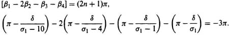
Solving, we obtain values of σ₁ at −0.45, −2.25, −4, and −12.5. the interpretation of these roots is the same as with the first method.

Rule 8. The intersection of the root locus and the imaginary axis can be determined by applying the Routh–Hurwitz stability criterion to the characteristic equation:

s⁴ + 9s³ + 24s² + (16 + 1.6K)s + 16K = 0.

Unfortunately, the Routh–Hurwitz method for a fourth-order system can given two possible answers. For example, in this problem, possible values of K where the root locus intersects the imaginary axis are 125 (from the second row) and 3.167 (from the third row). An alternative technique, which overcomes this problem, is to first solve for the frequencies where the locus intersects the imaginary axis, and then obtain the maximum values of gain from this expression. Letting s = jω, the characteristic equation becomes

The frequencies where the locus crosses the imaginary axis can be calculated from the real or the imaginary part of Eq. (6.168). Using the real part,

and using the imaginary part,

Solving Eqs. (6.169) and (6.170) simultaneously, we obtain

K_max = 3.167

or

k_max = 1.9794.

and the system is stable for 0 < K < 3.167. Substituting K_max = 3.167 into Eq. (6.170), we obtain

as the frequency of crossover of the imaginary axis.

Rule 9. This rule does not apply to this problem.

Rule 10. This rule shows that as certain of the loci turn to the right, others turn to the left to ensure that the sum of the roots is a constant.

Rule 11. This rule does not apply to this problem, because the problem does not require the calculation of gains along the locus.

Rule 12. The root locus does not cross itself.

The root locus of this system obtained using the 12 rules of construction is illustrated in Figure 6.61a. The root locus of this system obtained using the program MATLAB (see Section 6.17) is shown in Figure 6.61b, and is contained in the M-file that is part of my MCSTD Toolbox and it can be retrieved free from The MathWorks, Inc., anonymous FTP server at ftp://ftp.mathworks.com/pub/books/shinners.

Pertinent values of the root locus determined in this section and the rest of the book where the root locus is applied (for both positive and negative feedback) use the following special functions, which are part of my MCSTD Toolbox and are discussed in greater detail in Section 6.17: rlaxis; rlpoba; rootmag; rootangl. They determine the following:

1. rlaxis determines portions of the real axis that are part of the root locus.

   

   Figure 6.61(b)   Root locus obtained using MATLAB for same system illustrated in figure (a).

2. rlpoba determines the points of breakaway and break-in, and the values of gain at these points.
3. rootmag determines gain and values of the roots at a particular distance from the origin. (This is very valuable to us in Chapter 9 where the root locus is extended to discrete systems and we wish to find the gain and root values when the root locus crosses a unit circle that is the stability boundary for discrete systems.)
4. rootangl determines the gain and values of the roots at a particular angle from the origin. For example, to find K_max on the root locus and the value of s when it crosses the imaginary axis, the angle would be made equal to 90°. Another example is to determine the value of gain resulting for a particular value of ζ through the application of α = cos⁻¹(ζ).

These calculations are based on the root locus definitions, and are analytical and very accurate rather than using graphical techniques. My MCSTD Toolbox can be retrieved free from The MathWorks, Inc. anonymous FTP server at ftp://ftp.mathworks.com/pub/books/shinners.

Example 3

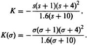
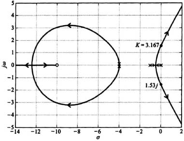
As a concluding third example for obtaining the root locus of a negative-feedback system, let us consider a unity-feedback system wehre

This system has three poles (two being a double pole) and one zero. The root locus of this system, illustrated in Figure 6.62, can be drawn on the basis of the rules of construction presented as follows:

Figure 6.62   Root locus of feedback system where .

Rule 1. There are three separate loci, as the characteristic equation is third order.

Rule 2. The root locus starts (K = 0) from the double poles located at −0.5, and at −2. One pole terminates (K = ∞) at the zero located at −4, and two loci terminate at zeros, which are located at infinity.

Rule 3. Complex portions of the root locus occur as complex-conjugate pairs, and the root locus is symmetrical with respect to the real axis.

Rule 4. The portions of the real axis between −2 and −4, and the point where the double poles exist at −0.5 are part of the root locus.

Rule 5. The loci approach infinity as K becomes large at angles given by

Rule 6. The intersection of the asymptotes and the real axis occur at

Rule 7. The point of breakaway is obviously at the double pole at −0.5. It is not necessary to apply this rule to find that fact.

Rule 8. The value of K_max and the intersection of the root locus and the imaginary axis can be found using the Routh–Hurwitz method as follows. The characteristic equation of this system is given by

s³ + 3s² + (2.25 + K)s + (4K + 0.5) = 0;

the resulting Routh–Hurwitz array is given by

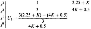
Setting the term in the third row U₁ = 0, we find that

K_max = 6.24.

Therefore, this system is stable for gains of

0 < K < 6.24.

To find the intersection of the root locus and the imaginary axis, we substitute s = jω and K = 6.24 into the characteristic equation. By setting the real or imaginary parts of the resulting equation equal to zero, we find that the intersection occurs at ±j2.92.

Rules 9, 10, 11, and 12 are not needed for this problem. Observe that the root locus plot of Figure 6.62 was obtained using the commercially available software package known as MATLAB (see Section 6.17), and is contained in the M-file that is part of my MCSTD Toolbox and can be retrieved free from The Math Works, Inc. anonymous FTP server at ftp://ftp.mathworks.com/pub/books/shinners.