
6.5. NYQUIST STABILITY CRITERION
The Nyquist stability criterion [5] is a very valuable tool that determines the degree of stability, or instability, of a feedback control system. In addition, it is the basis for other methods that are used to improve both the steady-state and the transient response of a feedback control system. Application of the Nyquist stability criterion requires a polar plot of the open-loop transfer function, G(jω)H(jω), which is usually referred to as the Nyquist diagram.
The Nyquist criterion determines the number of roots of the characteristic equation that have positive real parts from a polar plot of the open-loop transfer function, G(jω)H(jω), in the complex plane. Let us consider the characteristic equation
System stability can be determined from Eq. (6.54) by identifying the location of its roots in the complex plane. Assuming that G(s) and H(s), in their general form, are functions of s which are given by
and
then we can say that
Substituting Eq. (6.57) into Eq. (6.54), we obtain the following equivalent expression for F(s):
In terms of factors, we may rewrite Eq. (6.58) as
The factors s + zj are called the zero factors of F(s). This terminology is due to the fact that F(s) vanishes when s = −z1, −z2, and so on. The factors s + pi are called the pole factors of F(s). This terminology is due to the fact that F(s) is infinite when s = −p1 − p2, and so on.
Because F(s) is the denominator of the closed-loop system transfer function given by Eq. (6.6), we see that the zeros of F(s) are the poles of Eq. (6.6). Therefore, for a stable system, it is necessary the the zeros z1, z2, z3, … have negative real parts. The roots p1, p2, p3, have no real restrictions on them. As we shall shortly see, however, if we try to determine stability based on G(s)H(s) above, then a knowledge of the roots p1, p2, p3, … is also required. The only limitations of the Nyquist criterion are that the system be describable by a linear differential equation having constant coefficients.
The Nyquist diagram is a polar plot in the complex plane of G(s)H(s) as s follows the contour shown in Figure 6.8. Notice that the locus of s avoids poles of G(s)H(s) that lie anywhere on the imaginary axis by small semicircular paths passing to the right. These semicircular paths are assumed to have radii of infinitesimal magnitude. Any roots of the characteristic equation having positive real parts will lie within the contour shown in Figure 6.8.
Use is made of Cauchy’s [6] principle of the argument, which states that if function F(s) is analytic on and within a closed contour, except for a finite number of poles and zeros within the contour, then the number of times the origin of F(s) in the F plane is encircled as s traverses the closed contour once is equal to the number of zeros minus the number of poles of F(s), the poles and zeros being counted according to their multiplicity. In our particular case, the function F(s) equals 1 + G(s)H(s). Therefore, if 1 + G(s)H(s) is sketched for the contour defined by Figure 6.8, the number of times that 1 + G(s)H(s) encircles the origin equals the number of zeros minus the number of poles of 1 + G(s)H(s) for s in the right half-plane.
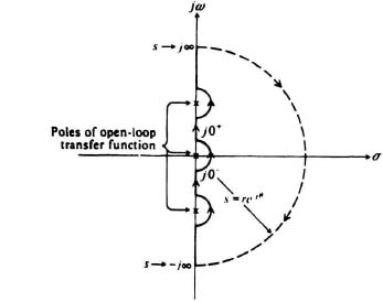
Figure 6.8 Locus of s in the complex plane for determining the Nyquist diagram.
Before we proceed to draw the Nyquist diagram, let us consider the polar plot of a sinusoidal transfer function G(jω). It is a plot of the vector G(jω), comprising the magnitude and phase angle of G(jω), on polar coordinates as ω is varied from zero to infinity. Figure 6.9 illustrates the plot of
as ω varies from zero to infinity. Observe from Figure 6.9 that each point on the polar plot of G(jω) represents the end point of a vector for a specific ω.
To illustrate the procedure using the Nyquist diagram, consider the system whose characteristic equation is given by
Its Nyquist diagram is shown in Figure 6.10. In part (a) of this figure, the Nyquist path for this system is illustrated. Note that its direction is clockwise, and it is defined by three sections: A, B, and C. Section A is defined from 0 ![]() ω
ω ![]() ∞; section B is defined from −∞
∞; section B is defined from −∞![]() ω
ω![]() 0; section C is defined from −∞
0; section C is defined from −∞![]() ω
ω![]() ∞. For part (b) of this figure, the Nyquist plot in the F(s) = 1 + G(s)H(s) plane corresponding to the Nyquist path defined in part (a) of the figure is illustrated. To obtain the direct polar plot of this function, we substitute s = jω into Eq. (6.61) as follows:
∞. For part (b) of this figure, the Nyquist plot in the F(s) = 1 + G(s)H(s) plane corresponding to the Nyquist path defined in part (a) of the figure is illustrated. To obtain the direct polar plot of this function, we substitute s = jω into Eq. (6.61) as follows:
Figure 6.10b represents the polar plot of 1 + G(s)H(s) for values of s along the imaginary axis. Sections A and B represent the polar plot of 1 + G(s)H(s) for values of s along the imaginary axis when −j∞![]() jω
jω![]() j∞. The dashed portion of the curve denotes the negative-frequency portion. The three sections corresponding to A, B, and C of both the Nyquist path (Figure 6.10a) and the Nyquist plot of Figure 6.10b are indicated. Notice that the semicircular section C of Figure 6.10a is only a point in Figure 6.10b. Observe that the F(s) locus encircles the origin twice. The G(s)H(s) locus is drawn in Figure 6.10c. Notice that the encirclement of origin by the plot of 1 + G(jω)H(jω) is equivalent to the encirclement of the −1, 0 point of the G(jω)H(jω) locus alone. Because it is easier to just draw the locus of G(jω)H(jω) rather than 1 + G(jω)H(jω), in practice we draw only the G(jω)H(jω) locus as in Figure 6.10c and determine the encirclement of the −1, 0 point. We start from ω = −∞, go through ω = 0, and end at ω = ∞, and we count the number of clockwise rotations of the vector in the G(jω)H(jω) plane. Observe that the plot of G(jω)H(jω) and the plot of G(−jω)H(−jω) are always symmetrical with each other about the real axis in the G(jω)H(jω) plane.
j∞. The dashed portion of the curve denotes the negative-frequency portion. The three sections corresponding to A, B, and C of both the Nyquist path (Figure 6.10a) and the Nyquist plot of Figure 6.10b are indicated. Notice that the semicircular section C of Figure 6.10a is only a point in Figure 6.10b. Observe that the F(s) locus encircles the origin twice. The G(s)H(s) locus is drawn in Figure 6.10c. Notice that the encirclement of origin by the plot of 1 + G(jω)H(jω) is equivalent to the encirclement of the −1, 0 point of the G(jω)H(jω) locus alone. Because it is easier to just draw the locus of G(jω)H(jω) rather than 1 + G(jω)H(jω), in practice we draw only the G(jω)H(jω) locus as in Figure 6.10c and determine the encirclement of the −1, 0 point. We start from ω = −∞, go through ω = 0, and end at ω = ∞, and we count the number of clockwise rotations of the vector in the G(jω)H(jω) plane. Observe that the plot of G(jω)H(jω) and the plot of G(−jω)H(−jω) are always symmetrical with each other about the real axis in the G(jω)H(jω) plane.

Figure 6.9 Polar plot of
![]()
as ω varies from zero to infinity.
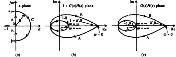
Figure 6.10 The Nyquist path (a) in the s-plane, and the Nyquist plots in the (b) 1 + G(s)H(s) and (c) G(s)H(s) planes for a system whose open-loop transfer function is given by
![]()
It is interesting to examine the 1 + G(s)H(s) and G(s)H(s) planes further as illustrated in Figure 6.11. Notice that the 1 + G(jω)H(jω) locus in the 1 + G(s)H(s) plane is measured from the origin to the locus. In the G(s)H(s) plane, the 1 + G(jω)H(jω) locus is the vector sum of the unit vector and the vector G(jω)H(jω). Therefore, observe that the 1 + G(jω)H(jω) vector drawn from the origin of the 1 + G(s)H(s) plane, and the 1 + G(jω)H(jω) vector drawn from the −1, 0 point in the G(s)H(s) plane are identical. The encirclement of the origin in the 1 + G(s)H(s) plane is, therefore, equivalent to encirclement of the −1 + j0 point in the G(s)H(s) plane.
With the Nyquist diagram sketched on a set of axes where the origin is shifted to the −1 + j0 point, the Nquist stability criterion can be stated algebraically as*

Figure 6.11 Polar plots of 1 + G(jω)H(jω) in the 1 + G(s)H(s) plane and G(jω)H(jω) in the G(s)H(s) plane for
![]()
where N is the number of clockwise encirclements of the −1 + j0 point by the Nyquist locus, P is the number of poles of the open-loop transfer function G(s)H(s) having positive real parts, and Z is the number of roots of the characteristic equation having positive real parts (Z must equal zero for stability). In most practical cases, the open-loop transfer function is in itself stable and P would equal zero. Because Z must equal zero for stability, N must equal zero for these practical systems.
For the example of Eq. (6.61) analyzed in Figure 6.10, G(s)H(s) does not have any poles in the right half-plane. Therefore, P = 0, and Z = N. Because the plot of Figure 6.10c shows two clockwise encirclements of the −1, 0 point, N = 2, and Z also equals 2, which means that there are two roots of the characteristic equation in the right half-plane. Therefore, the system is unstable. To stabilize this system, the gain K would have to be reduced, or a frequency-sensitive network would be added, until there were no encirclements of the −1, 0 point.
For cases where there exist one or more poles at the origin of the s-plane, the mapping from the s-plane to the G(s)H(s) plane is a little more difficult. As indicated in Figure 6.12a, all poles on the imaginary axis must be bypassed with small semi-circular paths. To illustrate the technique for this case, an open-loop transfer function containing a pure integration will be analyzed.
Figure 6.12a illustrates a polar plot, corresponding to the contour defined by Figure 6.8, for a system whose open-loop transfer function is given by
To obtain the direct polar plot of this function, we substitute s = jω into Eq. (6.64) as follows:
Figure 6.12b represents the polar plot of G(s)H(s) for the path shown in Figure 6.12a. The dashed portion of the curve denotes the negative-frequency portion. Notice that the polar plot for negative frequencies is the conjugate of the positive portion.
In part (a) of Figure 6.12, the Nyquist path for this system is illustrated. It is defined by four sections. Section AB is defined from 0+![]() ω
ω![]() ∞; section EFGHA is defined from 0−
∞; section EFGHA is defined from 0−![]() ω
ω![]() 0+; section DE is defined from −∞
0+; section DE is defined from −∞![]() ω
ω![]() 0−; section DCB is defined from −∞
0−; section DCB is defined from −∞![]() ω
ω![]() ∞. The plots of sections AB, DE, and DCB are similar in Figure 6.12a to that in Figure 6.10a. Notice that semicircular section DCB in Figure 6.12a is only a point in Figure 6.12b. However, the detour of the origin by path EFGHA in Figure 6.12a is new, and the procedure for obtaining it is as follows. The path along the imaginary axis in the vicinity of the origin is modified to be a semicircle of infinitesimal radius δ in the positive half-plane in order to avoid passing through this pole on the imaginary axis at the origin (see Figure 6.8). For this semicircular portion of the path, from j0− to j0+, s = δejθ, where δ → 0 and −π/2
∞. The plots of sections AB, DE, and DCB are similar in Figure 6.12a to that in Figure 6.10a. Notice that semicircular section DCB in Figure 6.12a is only a point in Figure 6.12b. However, the detour of the origin by path EFGHA in Figure 6.12a is new, and the procedure for obtaining it is as follows. The path along the imaginary axis in the vicinity of the origin is modified to be a semicircle of infinitesimal radius δ in the positive half-plane in order to avoid passing through this pole on the imaginary axis at the origin (see Figure 6.8). For this semicircular portion of the path, from j0− to j0+, s = δejθ, where δ → 0 and −π/2![]() θ
θ![]() π/2. Therefore, for s → 0, Eq. (6.64) becomes
π/2. Therefore, for s → 0, Eq. (6.64) becomes

Observe that the magnitude of K/δ → ∞ as δ → 0, and α = −θ goes from π/2 to −π/2 as the directed segment s goes from ![]() to
to ![]() This implies that the end points from ω → 0− and ω → 0+ in Figure 6.12b are joined by a semicircle of infinite radius in the first and fourth quadrants because as ω goes from 0− to 0+ in the s-plane (θ goes 180° counterclockwise), in the G(s)H(s) plane the locus has to go 180° clockwise in going from ω = 0− to 0+ because θ = −α in Eq. (6.66).
This implies that the end points from ω → 0− and ω → 0+ in Figure 6.12b are joined by a semicircle of infinite radius in the first and fourth quadrants because as ω goes from 0− to 0+ in the s-plane (θ goes 180° counterclockwise), in the G(s)H(s) plane the locus has to go 180° clockwise in going from ω = 0− to 0+ because θ = −α in Eq. (6.66).
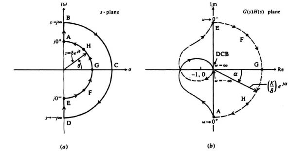
Figure 6.12 The Nyquist path in the s-plane (a), and the Nyquist plot in the G(s)H(s) plane (b) for a system whose open-loop transfer function is given by
![]()
Analysis of the Nyquist plot in Figure 6.12b indicates that there are two clockwise encirclements of the −1, 0 point. Therefore, N = 2 in Eq. (6.23), where
N = Z − P.
Because none of the poles of the open-loop transfer function are in the right half of the s-plane (P = 0), then
2 = Z − 0, Z = 2,
and there are two roots of the characteristic equation in the right half-plane. Therefore, this system is unstable for the value of K chosen. We could stabilize this system by reducing its gain K or adding a frequency-sensitive network until there were no encirclements of the −1, 0 point.
Figure 6.13 illustrates several examples of application of the Nyquist stability criterion using the relationship given by Eq. (6.63). In all cases, the values of the open-loop transfer function G(s)H(s) are shown together with the values of N, P, and Z. Notice that those systems whose Nyquist diagrams are illustrated in parts (a)–(d) are open-loop stable, whereas those in parts (e) and (f) are open-loop unstable. The systems illustrated in parts (a), (d), and (e) are closed-loop stable, whereas the systems illustrated in parts (b), (c) and (f) are closed-loop unstable.
It is quite clear that a good picture of a system’s margin of stability can be obtained from the Nyquist diagram. The proximity of the G(s)H(s) locus to the −1 + j0 point is an indication of relative stability. The farther away the locus is from this point, the greater the margin of stability. One conventional measure of the relative degree of stability is the distance two points on the G(s)H(s) locus are from the point −1 + j0. This is illustrated in Figure 6.14 by the points A and B.
Point A is defined by the intersection of the G(s)H(s) locus and the unit circle. Obviously, the magnitude of G(s)H(s) at point A is unity and is denoted by [G(jω)H(jω)]1 in Figure 6.14. The angle of [G(jω)H(jω)]1 with respect to the positive real axis is designated as θ. The phase margin γ is defined as the angle which [G(jω)H)(jω)]1 makes with respect to the negative real axis. It is related to θ (which is a negative angle) by the equation
A positive value of phase margin indicates stability, and a negative value of phase margin indicates instability. A zero value of phase margin indicates that the G(s)H(s) locus passes through the −1 + j0 point. The phase margin tells us how shy G(s)H(s) is of −180° when its magnitude is 1. (Remember, from Eq. (6.7), that we do not want G(s)H(s) = −1.) The magnitude of +γ indicates the relative degree of stability. Usually, a desirable value of γ is between 30° and 60°. It has been shown that the phase margin is approximately related to the damping ratio in second-order systems by the following approximation [6]
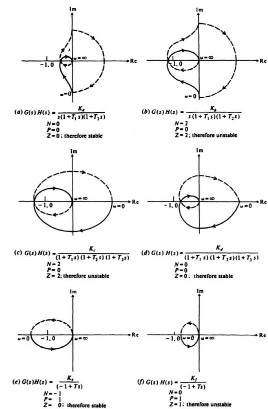
Figure 6.13 Examples of typical Nyquist diagrams.
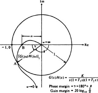
Figure 6.14 Definition of phase and gain margins.
Therefore, a damping factor of 0.5 requires a phase margin of approximately 50°.
The point B is defined by the intersection of the G(s)H(s) locus and the negative real axis. The gain margin is defined as the reciprocal of the magnitude of the G(s)H(s) locus at point B. For the configuration illustrated in Figure 6.14, the gain margin equals 1/α. The significance of the gain margin is that the system gain could be increased by a factor of 1/α before the G(s)H(s) locus would intersect the −1 + j0 point. A value of gain margin greater than unity indicates stability; a gain margin smaller than unity indicates instability. The magnitude of the gain margin indicates the relative degree of stability. Gain margin is conventionally expressed in decibels as follows:
For example, if α = 0.5, the gain margin is 6 dB. Usually, a desirable value of gain margin is between 4 and 12 dB. It is important to recognize that if the G(jω)H(jω) locus intersects the −1, 0 point, then the roots of the characteristic equation are located on the imaginary axis, and the phase and gain margins are zero. This should be avoided in practical control systems. The gain margin tells us how shy G(s)H(s) is of 1 when its phase is −180°. (Remember, from Eq. (6.7), that we do not want G(s)H(s) = −1.)
One important issue to be considered is that of conditionally stable systems. If Figure 6.14 is examined, the erroneous impression can be obtained that decrease in gain will always cause a system to become stable. This is not always true, as illustrated in Figure 6.15. Here, if the gain is decreased, point B will move to enclose the −1 + j0 point and the system will become unstable.
On the other hand, if the gain is increased, then point A will move to enclose the −1 + j0 point and the system will become unstable. Observe from the Nyquist diagram illustrated in Figure 6.15 that this control system is stable even though it appears that the −1, 0 point is enclosed. This is because the inner encirclement of the −1, 0 point, BCAD, is counterclockwise while the outer encirclements of the −1, 0 point, EHGF, is clockwise. Therefore, the net encirclements of the −1, 0 point is zero.
Some control systems have two or more phase crossover frequencies as illustrated in the Nyquist diagram of Figure 6.16. The phase margin for such a control system is measured at the highest gain crossover frequency.

Figure 6.15 Nyquist diagram of a conditionally stable system containing two gain margins.

Figure 6.16 The Nyquist diagram of a control system having three gain crossover frequencies.
Conditionally stable control systems containing multiple gain margins are discussed further in Section 6.14 from the viewpoints of the Bode diagram, and the root locus in Section 6.19.
Section 6.6 describes the approach for obtaining the Nyquist diagram using MATLAB. These Nyquist diagrams are contained in the M-files (that are part of my Modern Control System Theory and Design Toolbox) that can be retrieved free from The MathWorks, Inc. anonymous FTP server at ftp://ftp.mathworks.com/pub/books/shinners.