Search in book...
Toggle Font Controls
Create new playlist

Name your new playlist

Playlist description (optional)
Sign In

Email address

Password

Forgot Password?

or

Continue with Facebook

Continue with Google
Sign Up

Full Name

Email address

Confirm Email Address

Password

or

Continue with Facebook

Continue with Google

10.1 Graphs of `y` = `a` sin `x` and `y` = `a` cos `x`

Graphs of $y = \sin x$ $y = \sin x$ and $y = a \cos x$ $y = a \cos x$ • Amplitude • Graphs of $y = a \sin x$ $y = a \sin x$ and $y = a \cos x$ $y = a \cos x$

When plotting and sketching the graphs of the trigonometric functions, it is normal to express the angle in radians. By using radians, both the independent variable and the dependent variable are real numbers. If necessary, review Section 8.3 on radian measure of angles.

NOTE

[Therefore, it is necessary to be able to readily use angles expressed in radians.]

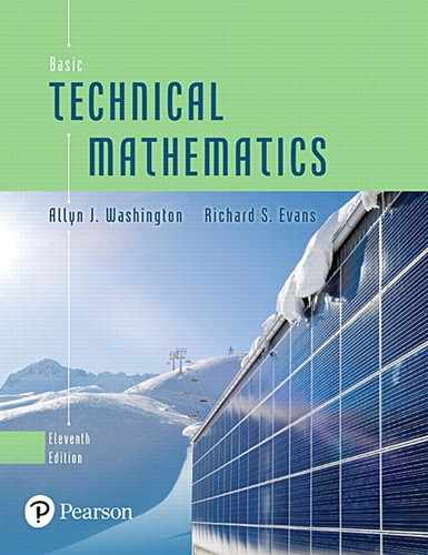
In this section, the graphs of the sine and cosine functions are shown. We begin by making a table of values of x and y for the function $y = \sin x,$ $y = \sin x,$ where x and y are used in the standard way as the independent variable and dependent variable. We plot the points to obtain the graph in Fig. 10.1.

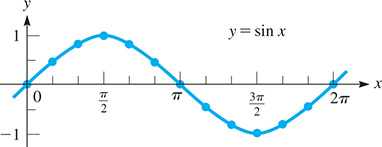
The graph is y = sine of x, which is a curve that oscillates about y = 0 with amplitude 1, period 2 pi, maximum (pi over 2, 1), and minimum (3 pi over 2, negative 1). — Fig. 10.1

Figure 10.1 Full Alternative Text

`x`	0	$\frac{π}{6}$ $\frac{π}{6}$	$\frac{π}{3}$ $\frac{π}{3}$	$\frac{π}{2}$ $\frac{π}{2}$	$\frac{2 π}{3}$ $\frac{2 π}{3}$	$\frac{5 π}{6}$ $\frac{5 π}{6}$	$π$ $π$
`y`	0	0.5	0.87	1	0.87	0.5	0

`x`	$\frac{7 π}{6}$ $\frac{7 π}{6}$	$\frac{4 π}{3}$ $\frac{4 π}{3}$	$\frac{3 π}{2}$ $\frac{3 π}{2}$	$\frac{5 π}{3}$ $\frac{5 π}{3}$	$\frac{11 π}{6}$ $\frac{11 π}{6}$	$2 π$ $2 π$
`y`	$- 0.5$ $- 0.5$	$- 0.87$ $- 0.87$	$- 1$ $- 1$	$- 0.87$ $- 0.87$	$- 0.5$ $- 0.5$	0

The graph of $y = \cos x$ $y = \cos x$ may be drawn in the same way. The next table gives values for plotting the graph of $y = \cos x,$ $y = \cos x,$ and the graph is shown in Fig. 10.2.

The graph is the curve y = cosine of x which oscillates about y = 0 with amplitude 1, period 2 pi, maximum (0, 1), and minimum (pi, negative 1). The curve rises and falls through points in the table following Figure 10.2. — Fig. 10.2

`x`	0	$\frac{π}{6}$ $\frac{π}{6}$	$\frac{π}{3}$ $\frac{π}{3}$	$\frac{π}{2}$ $\frac{π}{2}$	$\frac{2 π}{3}$ $\frac{2 π}{3}$	$\frac{5 π}{6}$ $\frac{5 π}{6}$	$π$ $π$
`y`	1	0.87	0.5	0	$- 0.5$ $- 0.5$	$- 0.87$ $- 0.87$	$- 1$ $- 1$

`x`	$\frac{7 π}{6}$ $\frac{7 π}{6}$	$\frac{4 π}{3}$ $\frac{4 π}{3}$	$\frac{3 π}{2}$ $\frac{3 π}{2}$	$\frac{5 π}{3}$ $\frac{5 π}{3}$	$\frac{11 π}{6}$ $\frac{11 π}{6}$	$2 π$ $2 π$
`y`	$- 0.87$ $- 0.87$	$- 0.5$ $- 0.5$	0	0.5	0.87	1

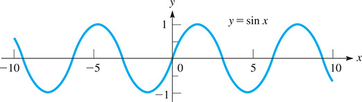
The graphs are continued beyond the values shown in the tables to indicate that they continue indefinitely in each direction. To show this more clearly, in Figs. 10.3 and 10.4, note the graphs of $y = \sin x$ $y = \sin x$ and $y = \cos x$ $y = \cos x$ from $x = - 10$ $x = - 10$ to $x = 10 .$ $x = 10 .$

The curve y = sine of x oscillates about y = 0 with amplitude 1, period 6.28, and maximum (1.57, 1). All data are approximate. — Fig. 10.3

The curve y = cosine of x oscillates about y = 0 with amplitude 1, period 2 pi, and a maximum at (0, 1). The x-axis is in increments of 5. — Fig. 10.4

From these tables and graphs, it can be seen that the graphs of $y = \sin x$ $y = \sin x$ and $y = \cos x$ $y = \cos x$ are of exactly the same shape (called sinusoidal), with the cosine curve displacement $π / 2$ $π / 2$ units to the left of the sine curve. The shape of these curves should be recognized readily, with special note as to the points at which they cross the axes. This information will be especially valuable in sketching similar curves, because the basic sinusoidal shape remains the same.

NOTE

[It will not be necessary to plot numerous points every time we wish to sketch such a curve. A few key points will be enough.]

AMPLITUDE

To obtain the graph of $y = a \sin x,$ $y = a \sin x,$ note that all the y-values obtained for the graph of $y = \sin x$ $y = \sin x$ are to be multiplied by the number a. In this case, the greatest value of the sine function is $| a | .$ $| a | .$ The number $| a |$ $| a |$ is called the amplitude of the curve and represents the greatest y-value of the curve. Also, the curve will have no value less than $- | a | .$ $- | a | .$ This is true for $y = a \cos x$ $y = a \cos x$ as well as $y = a \sin x .$ $y = a \sin x .$

EXAMPLE 1 Plot graph of `y` = `a` sin `x`

Plot the graph of $y = 2 \sin x .$ $y = 2 \sin x .$

Because $a = 2,$ $a = 2,$ the amplitude of this curve is $| 2 | = 2 .$ $| 2 | = 2 .$ This means that the maximum value of y is 2 and the minimum value is $y = - 2 .$ $y = - 2 .$ The table of values follows, and the curve is shown in Fig. 10.5.

A curve oscillates about y = 0 with amplitude 2. The amplitude is the distance from the line of oscillation to the maximum or minimum. — Fig. 10.5

`x`	0	$\frac{π}{6}$ $\frac{π}{6}$	$\frac{π}{3}$ $\frac{π}{3}$	$\frac{π}{2}$ $\frac{π}{2}$	$\frac{2 π}{3}$ $\frac{2 π}{3}$	$\frac{5 π}{6}$ $\frac{5 π}{6}$	$π$ $π$
`y`	0	1	1.73	2	1.73	1	0

`x`	$\frac{7 π}{6}$ $\frac{7 π}{6}$	$\frac{4 π}{3}$ $\frac{4 π}{3}$	$\frac{3 π}{2}$ $\frac{3 π}{2}$	$\frac{5 π}{3}$ $\frac{5 π}{3}$	$\frac{11 π}{6}$ $\frac{11 π}{6}$	$2 π$ $2 π$
`y`	$- 1$ $- 1$	$- 1.73$ $- 1.73$	$- 2$ $- 2$	$- 1.73$ $- 1.73$	$- 1$ $- 1$	0

EXAMPLE 2 Plot graph of `y` = `a` cos `x`

Plot the graph of $y = - 3 \cos x .$ $y = - 3 \cos x .$

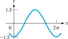
In this case, $a = - 3,$ $a = - 3,$ and this means that the amplitude is $| - 3 | = 3 .$ $| - 3 | = 3 .$ Therefore, the maximum value of y is 3, and the minimum value of y is $- 3 .$ $- 3 .$ The table of values follows, and the curve is shown in Fig. 10.6.

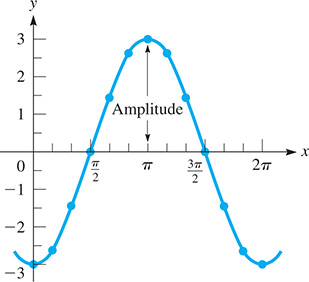
A curve rises through (0, negative 3) and (pi over 2, 0) to (pi, 3), then falls through (3 pi over 2, 0) to (2 pi, negative 3). The amplitude is from the x-axis to (pi, 3). — Fig. 10.6

`x`	0	$\frac{π}{6}$ $\frac{π}{6}$	$\frac{π}{3}$ $\frac{π}{3}$	$\frac{π}{2}$ $\frac{π}{2}$	$\frac{2 π}{3}$ $\frac{2 π}{3}$	$\frac{5 π}{6}$ $\frac{5 π}{6}$	$π$ $π$
`y`	$- 3$ $- 3$	$- 2.6$ $- 2.6$	$- 1.5$ $- 1.5$	0	1.5	2.6	3

`x`	$\frac{7 π}{6}$ $\frac{7 π}{6}$	$\frac{4 π}{3}$ $\frac{4 π}{3}$	$\frac{3 π}{2}$ $\frac{3 π}{2}$	$\frac{5 π}{3}$ $\frac{5 π}{3}$	$\frac{11 π}{6}$ $\frac{11 π}{6}$	$2 π$ $2 π$
`y`	2.6	1.5	0	$- 1.5$ $- 1.5$	$- 2.6$ $- 2.6$	$- 3$ $- 3$

NOTE

[Note that the effect of the negative sign with the number a is to invert the curve about the x-axis.]

From the previous examples, note that the function $y = a \sin x$ $y = a \sin x$ has zeros for $x = 0, π, 2 π$ $x = 0, π, 2 π$ and that it has its maximum or minimum values for $x = π / 2, 3 π / 2 .$ $x = π / 2, 3 π / 2 .$ The function $y = a \cos x$ $y = a \cos x$ has its zeros for $x = π / 2, 3 π / 2$ $x = π / 2, 3 π / 2$ and its maximum or minimum values for $x = 0, π, 2 π .$ $x = 0, π, 2 π .$ This is summarized in Table 10.1. Therefore, by knowing the general shape of the sine curve, where it has its zeros, and what its amplitude is, we can rapidly sketch curves of the form $y = a \sin x$ $y = a \sin x$ and $y = a \cos x .$ $y = a \cos x .$

Table 10.1

$x = 0, π, 2 π$ $x = 0, π, 2 π$		$\frac{π}{2}, \frac{3 π}{2}$ $\frac{π}{2}, \frac{3 π}{2}$
$y = a \sin x$ $y = a \sin x$	zeros	max. or min.
$y = a \cos x$ $y = a \cos x$	max. or min.	zeros

Because the graphs of $y = a \sin x$ $y = a \sin x$ and $y = a \cos x$ $y = a \cos x$ can extend indefinitely to the right and to the left, we see that the domain of each is all real numbers. We should note that the key values of $x = 0, π / 2, π, 3 π / 2,$ $x = 0, π / 2, π, 3 π / 2,$ and $2 π$ $2 π$ are those only for x from 0 to $2 π .$ $2 π .$ Corresponding values ( $x = 5 π / 2, 3 π,$ $x = 5 π / 2, 3 π,$ and their negatives) could also be used. Also, from the graphs, we can readily see that the range of these functions is $- | a | \leq f (x) \leq | a | .$ $- | a | \leq f (x) \leq | a | .$

EXAMPLE 3 Using key values to sketch graph

Sketch the graph of $y = 40 \cos x .$ $y = 40 \cos x .$

First, we set up a table of values for the points where the curve has its zeros, maximum points, and minimum points:

`x`	0	$\frac{π}{2}$ $\frac{π}{2}$	$π$ $π$	$\frac{3 π}{2}$ $\frac{3 π}{2}$	$2 π$ $2 π$
`y`	40 max.	0	$- 40 min .$ $- 40 min .$	0	40 max.

Now, we plot these points and join them, knowing the basic sinusoidal shape of the curve. See Fig. 10.7.

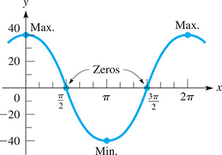
A curve oscillates about y = 0 with amplitude 40. It has a maximums (0, 40) and (2 pi, 40), zeros at (pi over 2, 0) and (3 pi over 2), and minimum (pi, negative 40). — Fig. 10.7

The graphs of $y = a \sin x$ $y = a \sin x$ and $y = a \cos x$ $y = a \cos x$ can be displayed easily on a calculator. In the next example, we see that the calculator displays the features of the curve we should expect from our previous discussion.

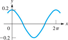
EXAMPLE 4 Displaying graphs on calculator—water wave

A certain water wave can be represented by the equation $y = - 2 \sin x$ $y = - 2 \sin x$ (measurements in ft). Display the graph on a calculator.

Using radian mode on the calculator, Fig. 10.8 shows the calculator view for the key values in the following table:

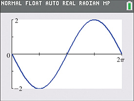
A curve oscillates about y = 0 with amplitude 2, period 2 pi, zeros (0, 0), (pi, 0), and (2 pi, 0), minimum (pi over 2, negative 2), and maximum (3 pi over 2, 2). — Fig. 10.8

`x`	0	$\frac{π}{2}$ $\frac{π}{2}$	$π$ $π$	$\frac{3 π}{2}$ $\frac{3 π}{2}$	$2 π$ $2 π$
`y`	0	$- 2 min .$ $- 2 min .$	0	2 max.	0

We see the amplitude of 2 and the effect of the negative sign in inverting the curve.

Exercises 10.1

In Exercises 1 and 2, graph the function if the given changes are made in the indicated examples of this section.

In Example 2, if the sign of the coefficient of cos x is changed, plot the graph of the resulting function.
In Example 4, if the sign of the coefficient of sin x is changed, display the graph of the resulting function.

In Exercises 3–6, complete the following table for the given functions and then plot the resulting graphs.

`x`	$- π$ $- π$	$- \frac{3 π}{4}$ $- \frac{3 π}{4}$	$- \frac{π}{2}$ $- \frac{π}{2}$	$- \frac{π}{4}$ $- \frac{π}{4}$	0	$\frac{π}{4}$ $\frac{π}{4}$	$\frac{π}{2}$ $\frac{π}{2}$	$\frac{3 π}{4}$ $\frac{3 π}{4}$	$π$ $π$
`y`

`x`	$\frac{5 π}{4}$ $\frac{5 π}{4}$	$\frac{3 π}{2}$ $\frac{3 π}{2}$	$\frac{7 π}{4}$ $\frac{7 π}{4}$	$2 π$ $2 π$	$\frac{9 π}{4}$ $\frac{9 π}{4}$	$\frac{5 π}{2}$ $\frac{5 π}{2}$	$\frac{11 π}{4}$ $\frac{11 π}{4}$	$3 π$ $3 π$
`y`

$y = \sin x$ $y = \sin x$
$y = \cos x$ $y = \cos x$
$y = - 3 \cos x$ $y = - 3 \cos x$
$y = - 4 \sin x$ $y = - 4 \sin x$

In Exercises 7–22, give the amplitude and sketch the graphs of the given functions. Check each using a calculator.

$y = 3 \sin x$ $y = 3 \sin x$
$y = 15 \sin x$ $y = 15 \sin x$
$y = \frac{5}{2} \sin x$ $y = \frac{5}{2} \sin x$
$y = 35 \sin x$ $y = 35 \sin x$
$y = 200 \cos x$ $y = 200 \cos x$
$y = 0.25 \cos x$ $y = 0.25 \cos x$
$y = 0.8 \cos x$ $y = 0.8 \cos x$
$y = \frac{3}{2} \cos x$ $y = \frac{3}{2} \cos x$
$y = - \sin x$ $y = - \sin x$
$y = - 30 \sin x$ $y = - 30 \sin x$
$y = - 1500 \sin x$ $y = - 1500 \sin x$
$y = - 0.2 \sin x$ $y = - 0.2 \sin x$
$y = - 4 \cos x$ $y = - 4 \cos x$
$y = - 8 \cos x$ $y = - 8 \cos x$
$y = - 50 \cos x$ $y = - 50 \cos x$
$y = - 0.4 \cos x$ $y = - 0.4 \cos x$

Although units of $π$ $π$ are convenient, we must remember that $π$ $π$ is only a number. Numbers that are not multiples of $π$ $π$ may be used. In Exercises 23–26, plot the indicated graphs by finding the values of y that correspond to values of x of 0, 1, 2, 3, 4, 5, 6, and 7 on a calculator. (Remember, the numbers 0, 1, 2, and so on represent radian measure.)

$y = \sin x$ $y = \sin x$
$y = - 30 \sin x$ $y = - 30 \sin x$
$y = - 12 \cos x$ $y = - 12 \cos x$
$y = 2 \cos x$ $y = 2 \cos x$

In Exercises 27–32, solve the given problems.

Find the function and graph it for a function of the form $y = a \sin x$ $y = a \sin x$ that passes through $(π / 2, - 2) .$ $(π / 2, - 2) .$
Find the function and graph it for a function of the form $y = a \sin x$ $y = a \sin x$ that passes through $(3 π / 2, - 2) .$ $(3 π / 2, - 2) .$
The height (in ft) of a person on a ferris wheel above its center is given by $h = - 32 \cos t$ $h = - 32 \cos t$ where t is the time (in s). Graph one complete cycle of this function.
The horizontal displacement d (in m) of the bob on a large pendulum is $d = 5 \sin t,$ $d = 5 \sin t,$ where t is the time (in s). Graph two cycles of this function.
The graph displayed on an oscilloscope can be represented by $y = - 0.05 \sin x .$ $y = - 0.05 \sin x .$ Display this curve on a calculator.
The displacement y (in cm) of the end of a robot arm for welding is $y = 4.75 \cos t,$ $y = 4.75 \cos t,$ where t is the time (in s). Display this curve on a calculator.

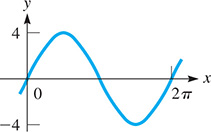
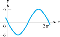
In Exercises 33–36, the graph of a function of the form $y = a \sin x$ $y = a \sin x$ or $y = a \cos x$ $y = a \cos x$ is shown. Determine the specific function of each.

Each ordered pair given in Exercises 37–40 is located on the graph of either $y = a \sin x$ $y = a \sin x$ or $y = a \cos x$ $y = a \cos x$ where the amplitude is $| a | = 2.50 .$ $| a | = 2.50 .$ Use the trace feature on a calculator to determine the equation of the function that contains the given point. (All points are located such that the x value is between $- π$ $- π$ and $π .$ $π .$ )

$(0.67, - 1.55)$ $(0.67, - 1.55)$
$(- 1.20, 0.90)$ $(- 1.20, 0.90)$
(2.07, 1.20)
$(- 2.47, - 1.55)$ $(- 2.47, - 1.55)$

Answers to Practice Exercise

`x`	0	$\frac{π}{2}$ $\frac{π}{2}$	$π$ $π$	$\frac{3 π}{2}$ $\frac{3 π}{2}$	$2 π$ $2 π$
`y`	0	$- 6 min .$ $- 6 min .$	0	6 max.	0

..................Content has been hidden....................

You can't read the all page of ebook, please click here login for view all page.

Table of Contents for 10.1 Graphs of y&#8201;=&#8201;a sin x and y&#8201;=&#8201;a cos x Graphs of y = a sin x and y = a cos x

Create new playlist

Sign In

Sign Up

Table of Contents for
10.1 Graphs of y = a sin x and y = a cos x Graphs of y = a sin x and y = a cos x