5.1 Linear Equations and Graphs of Linear Functions
Linear Equations • Solutions of Linear Equations • Linear Functions • Slope • Slope-Intercept Form • Sketching Lines by Intercepts • Linear Regression
In this chapter, we will discuss various techniques for solving systems of equations, which are groups of equations that contain more than one unknown. The methods we study assume that the equations are of a specific type, called linear equations. In this first section, we will define a linear equation and describe ways of graphing linear equations in two variables.
LINEAR EQUATIONS
An equation is called linear in a given set of variables if each term contains only one variable, to the first power, or is a constant. This is illustrated in the following example.
EXAMPLE 1 Identifying linear equations
Linear equations can have any number of unknowns (or variables). In Example 1, the equations in (a) and (b) are linear equations in two unknowns and the equation in (c) is a linear equation in three unknowns. The equations used throughout this chapter will be similar to the ones in (a)–(c).
EXAMPLE 2 Linear equations—Kirchhoff’s current and voltage laws
Kirchhoff’s current law states that the current going into any junction of an electric circuit equals the current going out. At the top junction in Fig. 5.1, this leads to
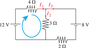
Fig. 5.1
Kirchhoff’s voltage law states that the sum of the voltages around any closed loop is zero. Going around the loop on the left in Fig. 5.1 (shown in blue) leads to
Both equations in this example are linear equations since the variables and occur only to the first power. Note that a third equation could be found by applying the voltage law to the closed loop on the right in Fig. 5.1.
The first method of solving a system of equations that we will discuss relies on graphing linear equations in two unknowns. Before taking this method up in Section 5.2, we will first develop additional ways of graphing these equations.
GRAPHING A LINEAR EQUATION IN TWO UNKNOWNS
A linear equation in two unknowns is an equation that can be written in the following form:
A solution of such an equation is a pair of numbers, one for each variable, that when substituted into the equation, makes the equation true. Therefore, each solution is an ordered pair that can be plotted as a point in the rectangular coordinate system. There are an infinite number of these ordered-pair solutions, which together form the graph of the equation. This is illustrated in the following example.
EXAMPLE 3 Graphing a linear equation in two unknowns
Graph the equation
We first need to find several pairs of numbers (x, y) that are solutions to the equation, meaning they make the equation true when x and y are substituted in. If we first solve for y to get the solutions are easier to find. We can substitute any number in for x and then find the corresponding value of y that makes the equation true. The resulting pair of numbers (x, y) is a solution to the equation, and when plotted, is one point on the graph. The table feature on a calculator can be used to find many solutions quickly, as shown in Fig. 5.2. All these pairs of values satisfy the original equation, meaning they make it true. When these points are plotted together, they form the graph of the equation as shown in Fig. 5.3. Note that the graph is a straight line. In general, all linear equations in two unknowns have graphs that are straight lines.

Fig. 5.2

Fig. 5.3
LINEAR FUNCTIONS AND SLOPE
For a linear equation in two unknowns, it is always possible to solve for one variable in terms of the other to put it in the form where m and b are constants (as we did in Example 3). Written this way, it is clear that y is a function of x, and thus, it is called a linear function. Another method for graphing a line is to interpret the values of m and b in this equation to obtain a graph of the line. To do this, one must first understand the concept of slope.
Consider the line that passes through points A, with coordinates and B, with coordinates in Fig. 5.4. Point C is horizontal from A and vertical from B. Thus, C has coordinates and there is a right angle at C. One way of measuring the steepness of this line is to find the ratio of the vertical distance to the horizontal distance between two points. Therefore, we define the slope of the line through two points as the difference in the y-coordinates divided by the difference in the x-coordinates. For points A and B, the slope m is

Fig. 5.4
CAUTION
Be very careful not to reverse the order of subtraction. is not equal to
The slope is often referred to as the rise (vertical change) over the run (horizontal change).
NOTE
[The slope of a vertical line, for which is undefined since the denominator of Eq. (5.2) is zero. Also, the slope of a horizontal line, for which is zero.]
EXAMPLE 4 Slope of line through two points
Find the slope of the line through the points and (5, 3).
In Fig. 5.5, we draw the line through the two given points. By taking (5, 3) as then is We may choose either point as but once the choice is made the order must be maintained. Using Eq. (5.2), the slope is
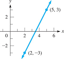
Fig. 5.5
The rise is 2 units for each unit (of run) in going from left to right.
EXAMPLE 5 Slope of line through two points
Find the slope of the line through and
In Fig. 5.6, we draw the line through these two points. By taking as and as the slope is

Fig. 5.6
The line falls 3 units for each 4 units in going from left to right.
We note in Example 1 that as x increases, y increases and the slope is positive. In Example 2, as x increases, y decreases and the slope is negative. Also, the larger the absolute value of the slope, the steeper is the line.
EXAMPLE 6 Slope and steepness of line
For each of the following lines shown in Fig. 5.7, we show the difference in the y-coordinates and in the x-coordinates between two points.
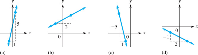
Fig. 5.7
In Fig. 5.7(a), a line with a slope of 5 is shown. It rises sharply.
In Fig. 5.7(b), a line with a slope of is shown. It rises slowly.
In Fig. 5.7(c), a line with a slope of is shown. It falls sharply.
In Fig. 5.7(d), a line with a slope of is shown. It falls slowly.
SLOPE-INTERCEPT FORM OF THE EQUATION OF A STRAIGHT LINE
We now show how the slope is related to the equation of a straight line. In Fig. 5.8, if we have two points, (0, b) and a general point (x, y), the slope is

Fig. 5.8
Simplifying this, we have or
In Eq. (5.3), m is the slope, and b is the y-coordinate of the point where the line crosses the y-axis. This point is the y-intercept of the line, and its coordinates are (0, b).
NOTE
[Equation (5.3) is the slope-intercept form of the equation of a straight line. The coefficient of x is the slope, and the constant is the ordinate of the y-intercept.]
The point (0, b) and simply b are both referred to as the y-intercept.
EXAMPLE 7 Slope-intercept form of equation
Use the slope and the y-intercept of the line to sketch its graph.
Because we can write this as
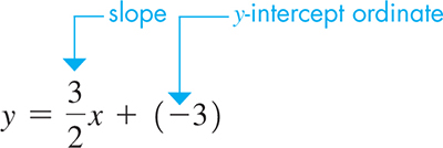
the slope is and the y-intercept is To graph, we start at and then move up 3 units and to the right by 2 units. See Fig. 5.9.
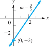
Fig. 5.9
EXAMPLE 8 Slope-intercept form of equation
Find the slope and the y-intercept of the line
We must first write the equation in slope-intercept form. Solving for y, we have
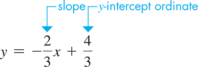
Therefore, the slope is and the y-intercept is the point See Fig. 5.10.

Fig. 5.10
EXAMPLE 9 Slope-intercept form—Fahrenheit and Celsius temperature
The equation relates degrees Fahrenheit (F) and degrees Celsius (C). This is a linear function in slope-intercept form. The F-intercept is (0, 32), which represents the freezing point of water The slope is meaning the Fahrenheit temperature rises 9 degrees for every 5 degrees of Celsius temperature. To graph this by hand, we can start at (0, 32) and then go up 9 units and to the right 5 units (see Fig. 5.11). This can also be graphed on a calculator by entering and then graphing with appropriate window settings (see Fig. 5.12).
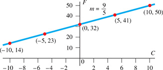
Fig. 5.11
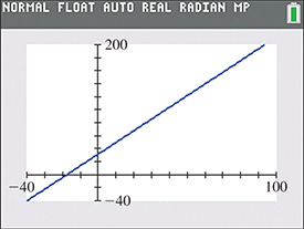
Fig. 5.12
SKETCHING LINES BY INTERCEPTS
Another way of sketching the graph of a straight line is to find two points on the line and then draw the line through these points. Two points that are easily determined are those where the line crosses the y-axis and the x-axis. We already know that the point where it crosses the y-axis is the y-intercept.
NOTE
[In the same way, the point where a line crosses the x-axis is called the x-intercept, and the coordinates of the x-intercept are (a, 0).]
The intercepts are easily found because one of the coordinates is zero. By setting and in turn, and finding the value of the other variable, we get the coordinates of the intercepts. This method works except when both intercepts are at the origin, and we must find one other point, or use the slope-intercept method. In using the intercept method, a third point should be found as a check. The next example shows how a line is sketched by finding its intercepts.
EXAMPLE 10 Sketching line by intercepts
Sketch the graph of the line by finding its intercepts and one check point. See Fig. 5.13.

Fig. 5.13
First, we let This gives us or This gives us the y-intercept, which is the point Next, we let which gives us or This means the x-intercept is the point (3, 0).
The intercepts are enough to sketch the line as shown in Fig. 5.13. To find a check point, we can use any value for x other than 3 or any value of y other than Choosing we find that This means that the point should be on the line. In Fig. 5.13, we can see that it is on the line.
Note that in order to graph this on a calculator, we must first solve for y to get Then we can enter and graph with appropriate window settings.
LINEAR REGRESSION
In Example 9, we saw that Fahrenheit and Celsius temperatures have an exact linear relationship. Sometimes when analyzing data, we find that two variables have an approximate linear relationship. This happens when the plotted data points are somewhat scattered, but generally follow a straight-line pattern. In these cases, a regression line can be used to model the data. A regression line is obtained from statistical methods that ensure it will be the line that best fits the data points. Many calculators can also be used to find regression lines, and the next example shows how this is done.
EXAMPLE 11 Linear regression—speed of sound versus temperature
In an experiment, the temperature (in °C) and the speed of sound in air (in m/s) were measured on seven days throughout the year as shown in the table:
| Temperature, T (°C) | 2.4 | 8.1 | 11.4 | 16.8 | 22.2 | ||
| Measured speed of sound, v (m/s) | 327 | 329 | 332 | 336 | 337 | 341 | 345 |
The statistical graphing features on a calculator can be used to make a scatterplot of the data as shown in Fig. 5.14(a). Since the points generally follow a straight line, we can use the feature to find the regression line, which is shown in Fig. 5.14(b). The result (after rounding to 3 decimal places) is This equation can be entered for and graphed through the scatterplot as shown in Fig. 5.14(c).
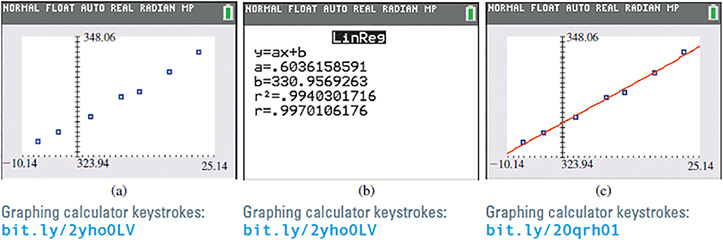
Fig. 5.14
The regression equation is in the form with and Thus, it is a linear function in slope-intercept form. Using the variables in our example, we can rewrite the regression line as
The regression equation can be used to predict the value of either variable if the other variable is known. For example, to predict the speed of sound in air with temperature 20.0°C, we have To predict the temperature that would result in a speed of sound of 334 m/s, we substitute 334 in for v and then solve for T, which yields
EXERCISES 5.1
In Exercises 1–4, answer the given questions about the indicated examples of this section.
In Example 3, what is the solution if
In Example 5, if the first y-coordinate is changed to what changes result in the example?
In the first line of Example 8, if is changed to what changes result in the example?
In the first line of Example 10, if is changed to what changes occur in the graph?
In Exercises 5–8, determine whether or not the given equation is linear.
In Exercises 9–12, determine whether or not the given pair of values is a solution to the given linear equation in two unknowns.
In Exercises 13–16, for each given value of x, determine the value of y that gives a solution to the given linear equation in two unknowns.
In Exercises 17–24, find the slope of the line that passes through the given points.
(1, 0), (3, 8)
In Exercises 25–32, sketch the line with the given slope and y-intercept.
In Exercises 33–40, find the slope and y-intercept of the line with the given equation and sketch the graph using the slope and y-intercept. A calculator can be used to check your graph.
In Exercises 41–48, find the x- and y-intercepts of the line with the given equation. Sketch the line using the intercepts. A calculator can be used to check the graph.
In Exercises 49–52, find the equation of the regression line for the given data. Then use this equation to make the indicated estimate. Round decimals in the regression equation to three decimal places. Round estimates to the same accuracy as the given data.
The following table gives the weld diameters d (in mm) and the shear strengths s (in kN/mm) for a sample of spot welds. Find the equation of the regression line, and then estimate the shear strength of a spot weld that has a diameter of 4.5 mm.
Diameter, d (mm) 4.2 4.4 4.6 4.8 5.0 5.2 5.4 Shear strength, s (kN/mm) 51 54 69 76 75 85 89 The following table gives the percentage p of adults living in households with only wireless telephone services, where t is the number of years after the year 2000. Find the equation of the regression line, and then estimate the percentage of adults living in households with only wireless telephone services in the year 2016.
Number of years after 2000, t 6 8 10 12 14 Percentage with only wireless phones, p (%) 10 16 25 34 43 The following data gives the diameter in inches (measured 4.5 ft above ground) and the volume of wood (in ) for a sample of black cherry trees. Find the equation of the regression line, and then estimate the volume of wood in a black cherry tree that has a diameter of 15.0 in.
Diameter, d (in.) 8.8 11.0 11.2 11.7 13.7 16.0 17.9 20.6 Volume, v 10.2 15.6 19.9 21.3 25.7 38.3 58.3 77.0 The following table gives the fraction f (as a decimal) of the total heating load of a certain system that will be supplied by a solar collector of area A (in ). Find the equation of the regression line, and then estimate the fraction of the heating load that will be supplied by a solar collector with area
Area, A 20 30 40 50 60 70 80 Fraction, f 0.22 0.30 0.37 0.44 0.50 0.56 0.61
In Exercises 53–56, solve the given problems.
Find the intercepts of the line
Find the intercepts of the line
Do the points and lie on the same straight line?
The points and (3, 7) are on the same straight line.
Find another point on the line for which .
Find another point on the line for which
In Exercises 57–62, sketch the indicated lines.
The diameter of the large end, d (in in.), of a certain type of machine tool can be found from the equation where l is the length of the tool. Sketch d as a function of l, for values of l to 10 in. See Fig. 5.15

Fig. 5.15
In mixing 85-octane gasoline and 93-octane gasoline to produce 91-octane gasoline, the equation is used. Sketch the graph.
Two electric currents, and (in mA), in part of a circuit in a computer are related by the equation Sketch as a function of These currents can be negative.
In 2009, it was estimated that about 4.1 billion text messages were sent each day in the United States, and in 2012 it was estimated that this number was 6.2 billion. Assuming the growth in texting is linear, set up a function for the number N of daily text messages and the time t in years, with being 2009. Sketch the graph for to
A plane cruising at 220 m/min starts its descent from 2.5 km at 150 m/min. Find the equation for its altitude h as a function of time t and sketch the graph for to
A straight ski run declines 80 m over a horizontal distance of 480 m. Find the equation for the height h of a skier above the bottom as a function of the horizontal distance d moved. Sketch the graph.
Answers to Practice Exercises
(5, 0),