13.7 Graphs on Logarithmic and Semilogarithmic Paper
Logarithmic Scale • Semilogarithmic (Semilog) Paper • Logarithmic (Log-Log) Paper
When constructing the graphs of some functions, one of the variables changes much more rapidly than the other. We saw this in graphing the exponential and logarithmic functions in Sections 13.1 and 13.2. The following example illustrates this point.
EXAMPLE 1 Graph of exponential function
Plot the graph of
Constructing the following table of values,
| x | 0 | 1 | 2 | 3 | 4 | 5 | |
| y | 1.3 | 4 | 12 | 36 | 108 | 324 | 972 |
we then plot these values as shown in Fig. 13.21(a).

Fig. 13.21
We see that as x changes from to 5, y changes much more rapidly, from about 1 to nearly 1000. Also, because of the scale that must be used, we see that it is not possible to show accurately the differences in the y-values on the graph.
Even a calculator cannot show the graph accurately for the values near if we wish to view all of this part of the curve. In fact, the calculator view shows the curve as being on the axis for these values, as we see in Fig. 13.21(b). Note in this figure that we have shown the same values of the range of the function as we did in Fig. 13.21(a).
It is possible to graph a function with a large change in values, for one or both variables, more accurately than can be done on the standard rectangular coordinate system. This is done by using a scale marked off in distances proportional to the logarithms of the values being represented. Such a scale is called a logarithmic scale. For example, and Thus, on a logarithmic scale, the 2 is placed 0.301 unit of distance from the 1 to the 10. Figure 13.22 shows a logarithmic scale with the numbers represented and the distance used for each.

Fig. 13.22
On a logarithmic scale, the distances between the integers are not equal, but this scale does allow for a much greater range of values and much greater accuracy for many of the values. There is another advantage to using logarithmic scales. Many equations that would have more complex curves when graphed on the standard rectangular coordinate system will have simpler curves, often straight lines, when graphed using logarithmic scales. In many cases, this makes the analysis of the curve much easier.
Zero and negative numbers do not appear on the logarithmic scale. In fact, all numbers used on the logarithmic scale must be positive, because the domain of the logarithmic function includes only positive real numbers. Thus, the logarithmic scale must start at some number greater than zero. This number is a power of 10 and can be very small, say, but it is positive.
If we wish to use a large range of values for only one of the variables, we use what is known as semilogarithmic, or semilog, graph paper. On this graph paper, only one axis (usually the y-axis) uses a logarithmic scale. If we wish to use a large range of values for both variables, we use logarithmic, or log-log, graph paper. Both axes are marked with logarithmic scales.
The following examples illustrate semilog and log-log graphs, which are used in many technical and scientific areas to display coordinates of plotted points more clearly.
EXAMPLE 2 Graph on semilogarithmic paper
Construct the graph of on semilogarithmic graph paper.
This is the same function as in Example 1, and we repeat the table of values:
| x | 0 | 1 | 2 | 3 | 4 | 5 | |
| y | 1.3 | 4 | 12 | 36 | 108 | 324 | 972 |
Again, we see that the range of y-values is large. When we plotted this curve on the rectangular coordinate system in Example 1, we had to use large units along the y-axis. This made the values of 1.3, 4, 12, and 36 appear at practically the same level. However, when we use semilog graph paper, we can label each axis such that all y-values are accurately plotted as well as the x-values.
The logarithmic scale is shown in cycles, and we must label the base line of the first cycle as 1 times a power of 10 (0.01, 0.1, 1, 10, 100, and so on) with the following cycle labeled with the next power of 10. The lines between are labeled with 2, 3, 4, and so on, times the proper power of 10. See the vertical scale in Fig. 13.23. We now plot the points in the table on the graph. The resulting graph is a straight line, as we see in Fig. 13.23. Taking logarithms of each side of the equation, we have
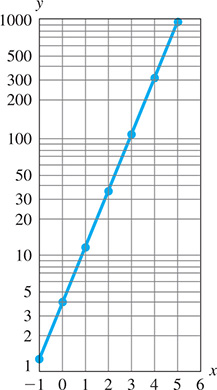
Fig. 13.23
However, because log y was plotted automatically (because we used semilogarithmic paper), the graph really represents
where and are constants, and therefore this equation is of the form which is a straight line (see Section 5.1).
The logarithmic scale in Fig. 13.23 has three cycles, because all values of three powers of 10 are represented.
EXAMPLE 3 Graph on logarithmic paper
Construct the graph of on logarithmic paper.
First, we solve for y and make a table of values. Considering positive values of x and y, we have
| x | 0.5 | 1 | 2 | 8 | 20 | |
| y | 4 | 1 | 0.25 | 0.0156 | 0.0025 |
We plot these values on log-log paper on which both scales are logarithmic, as shown in Fig. 13.24. We again see that we have a straight line. Taking logarithms of both sides of the equation, we have
If we let and we then have
which is the equation of a straight line, as shown in Fig. 13.24. Note, however, that not all graphs on logarithmic paper are straight lines.

Fig. 13.24
EXAMPLE 4 Graph on log-log paper—beam deflection
The deflection (in ft) of a certain cantilever beam as a function of the distance x (in ft) from one end is
If the beam is 20.0 ft long, plot a graph of d as a function of x on log-log paper.
Constructing a table of values, we have
| x (ft) | 1.00 | 1.50 | 2.00 | 3.00 | 4.00 |
| d (ft) | 0.00290 | 0.00641 | 0.0112 | 0.0243 | 0.0416 |
| x (ft) | 5.00 | 10.0 | 15.0 | 20.0 |
| d (ft) | 0.0625 | 0.200 | 0.338 | 0.400 |
Because the beam is 20.0 ft long, there is no meaning to values of x greater than 20.0 ft. The graph is shown in Fig. 13.25.
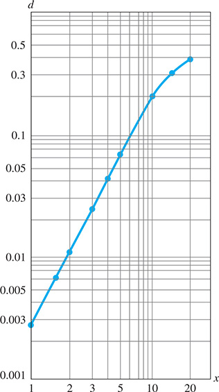
Fig. 13.25
Logarithmic and semilogarithmic paper may be useful for plotting data. Often, the data cover too large a range of values to be plotted on ordinary graph paper. The next example illustrates the use of semilogarithmic paper to plot data.
EXAMPLE 5 Excel scatterplot on semilog scale—transistors
The number of transistors in computer processors has increased dramatically over the years. The Excel spreadsheet in Fig. 13.26 shows some selected processors, the date of release, and the number of transistors. Also shown is a scatterplot of the data using a semilog scale. If plotted on a standard scale (see Fig. 13.27), the points prior to the year 2000 all appear to lie on the x-axis due to the fact that the transistor count has reached extremely high numbers in recent years. The semilog scale shows the data much more clearly.
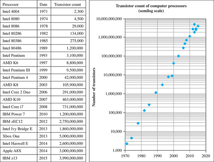
Fig. 13.26

Fig. 13.27
EXERCISES 13.7
In Example 2, change the 4 to 2 and then make the graph.
In Example 3, change the 1 to 4 and then make the graph.
On the moon, the distance s (in ft) a rock will fall due to gravity is Where t is the time (in s) of fall. Plot the graph of s as a function of t for on (a) a regular rectangular coordinate system and (b) a semilogarithmic coordinate system.
By pumping, the air pressure in a tank is reduced by 18% each second. Thus, the pressure p (in kPa) in the tank is given by where t is the time (in s). Plot the graph of p as a function of t for on (a) a regular rectangular coordinate system and (b) a semilogarithmic coordinate system.
Strontium-90 decays according to the equation where N is the amount present after t years and is the original amount. Plot N as a function of t on semilog paper if
The electric power P (in W) in a certain battery as a function of the resistance R (in ) in the circuit is given by Plot P as a function of R on semilog paper, using the logarithmic scale for R and values of R from to
The acceleration g (in ) produced by the gravitational force of Earth on a spacecraft is given by where r is the distance from the center of Earth to the spacecraft. On log-log paper, graph g as a function of r from (Earth’s surface) to (the distance to the moon).
In undergoing an adiabatic (no heat gained or lost) expansion of a gas, the relation between the pressure p (in kPa) and the volume v (in ) is On log-log paper, graph p as a function of v from to
The number of cell phone subscribers in the United States from 1994 to 2015 is shown in the following table. Plot N as a function of the year on semilog paper.
Year 1994 1997 2000 2003 2006 2009 2012 2015 24.1 55.3 109 159 233 275 300 359 The period T (in years) and mean distance d (given as a ratio of that of Earth) from the sun to the planets (Mercury, Venus, Earth, Mars, Jupiter, Saturn, Uranus, Neptune, Pluto) are given below. Plot T as a function of d on log-log paper. (Note that Pluto is currently considered to be a dwarf planet.)
Planet M V E M J S U N P d 0.39 0.72 1.00 1.52 5.20 9.54 19.2 30.1 39.5 T 0.24 0.62 1.00 1.88 11.9 29.5 84.0 165 249 The intensity level B (in dB) and the frequency f (in Hz) for a sound of constant loudness were measured as shown in the table that follows. Plot the data for B as a function of f on semilog paper, using the log scale for f.
f (Hz) 100 200 500 1000 2000 5000 10,000 B (dB) 40 30 22 20 18 24 30 The atmospheric pressure p (in kPa) at a given altitude h (in km) is given in the following table. On semilog paper, plot p as a function of h.
h
(km)0 10 20 30 40 p (kPa) 101 25 6.3 2.0 0.53 One end of a very hot steel bar is sprayed with a stream of cool water. The rate of cooling R (in °F/s) as a function of the distance d (in in.) from one end of the bar is then measured, with the results shown in the following table. On log-log paper, plot R as a function of d. Such experiments are made to determine the hardness of steel.
d (in.) 0.063 0.13 0.19 0.25 R (°F/s) 600 190 100 72 d (in.) 0.38 0.50 0.75 1.0 1.5 R (°F/s) 46 29 17 10 6.0 The magnetic intensity H (in A/m) and flux density B (in teslas) of annealed iron are given in the following table. Plot H as a function of B on log-log paper. (The unit tesla is named in honor of Nikola Tesla. See Chapter 20 introduction.)
B (T) 0.0042 0.043 0.67 1.01 H (A/m) 10 50 100 150 B (T) 1.18 1.44 1.58 1.72 H (A/m) 200 500 1000 10,000
In Exercises 39 and 40, plot the indicated semilogarithmic graphs for the following application.
In a particular electric circuit, called a low-pass filter, the input voltage is across a resistor and a capacitor, and the output voltage is across the capacitor (see Fig. 13.28). The voltage gain G (in dB) is given by
where

Fig. 13.28
Here, is the phase angle of For values of of 0.01, 0.1, 0.3, 1.0, 3.0, 10.0, 30.0, and 100, plot the indicated graphs. These graphs are called a Bode diagram for the circuit.
Calculate values of G for the given values of and plot a semilogarithmic graph of G vs.
Calculate values of (as negative angles) for the given values of and plot a semilogarithmic graph of