5.2 Systems of Equations and Graphical Solutions
System of Linear Equations • Solution of a System • Solution by Graphing • Using a Graphing Calculator • Inconsistent and Dependent Systems
In many applications, there is more than one unknown that we wish to solve for. To accomplish this, we must also have more than one equation that involves these unknowns. In fact, we need as many equations as there are unknowns. A group of two or more equations involving two or more unknowns is called a system of equations. In the remaining sections of this chapter, we will discuss various techniques for solving systems of linear equations. We begin by studying systems of two equations with two unknowns.
Two linear equations, each containing the same two unknowns,
are said to form a system of linear equations in two unknowns.
NOTE
[A solution of the system is a pair of numbers (x, y) that make both equations true.]
Except in special circumstances, there will only be one pair of numbers that make both equations true. The following two examples illustrate the meaning of a solution of a system.
EXAMPLE 1 Testing for solution of a system
Is (2, 8) a solution of the system ?
Substituting and into each equation, we get
Since both equations are true, is a solution of the system.
EXAMPLE 2 Testing for solution of a system—finding forces
Are the forces in the following system given by and ?
Substituting into the equations, we have
Since one of these equations is not true, is not a solution of the system.
SOLUTION BY GRAPHING
In Section 5.1, we saw that the graph of a linear equation in two unknowns is a straight line. Because a solution of a system of linear equations in two unknowns is a pair of values (x, y) that satisfies both equations, graphically the solution is given by the coordinates of the point of intersection of the two lines. This must be the case, for the coordinates of this point constitute the only pair of values to satisfy both equations. (In some special cases, there may be no solution; in others, there may be many solutions.See Examples 7 and 8.)
Therefore, when we solve a system of equations in two unknowns graphically, we must graph each line and determine the point of intersection. When doing this by hand, we often need to estimate the point of intersection. However, we will show in Example 5 that a calculator can be used to find this point very accurately.
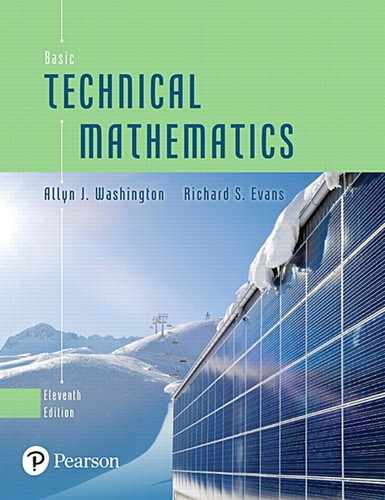
EXAMPLE 3 Determine the point of intersection
Solve the system of equations
Because each of the equations is in slope-intercept form, note that and for the first line and that and for the second line. Using these values, we sketch the lines, as shown in Fig. 5.16.
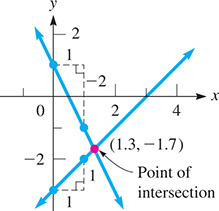
Fig. 5.16
From the figure, it can be seen that the lines cross at about the point
This means that the solution is approximately
(The exact solution is )
NOTE
[In checking the solution, be careful to substitute the values in both equations.]
Making these substitutions gives us
These values show that the solution checks. [The point is on the first line and almost on the second line. The difference in values when checking the values for the second line is due to the fact that the solution is approximate.]
EXAMPLE 4 Determine the point of intersection
Solve the system of equations
We could write each equation in slope-intercept form in order to sketch the lines. Also, we could use the form in which they are written to find the intercepts. Choosing to find the intercepts and draw lines through them, let then Therefore, the intercepts of the first line are the points (5, 0) and (0, 2). A third point is The intercepts of the second line are (2, 0) and A third point is Plotting these points and drawing the proper straight lines, we see that the lines cross at about (2.3, 1.1). [The exact values are ] The solution of the system of equations is approximately (see Fig. 5.17).
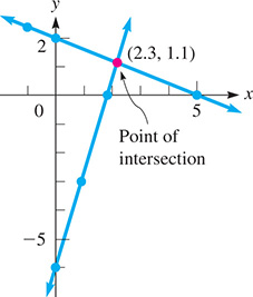
Fig. 5.17
Checking, we have
This shows the solution is correct to the accuracy we can get from the graph.
SOLVING SYSTEMS OF EQUATIONS USING A GRAPHING CALCULATOR
A calculator can be used to find the point of intersection with much greater accuracy than is possible by hand-sketching the lines. Once we locate the point of intersection, the features of the calculator allow us to get the accuracy we need.
EXAMPLE 5 Using a calculator to find points of intersection
Using a calculator, we now solve the systems of equations in Examples 3 and 4.
Solving the system for Example 3, let and Then display the lines as shown in Fig. 5.18(a). Then using the intersect feature of the calculator, we find (rounded to the nearest 0.001) that the solution is
Fig. 5.18
Solving the system for Example 4, let and Then display the lines as shown in Fig. 5.18(b). Then using the intersect feature, we find (rounded to the nearest 0.001) that the solution is
APPLICATIONS INVOLVING TWO LINEAR EQUATIONS
Linear equations in two unknowns are often useful in solving applied problems. Just as in Section 1.12, we must read the statement carefully in order to identify the unknowns and the information for setting up the equations.
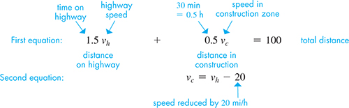
EXAMPLE 6 Solving a system—speed of a car
A driver traveled for 1.5 h at a constant speed along a highway. Then, through a construction zone, the driver reduced the car’s speed by 20 mi/h for 30 min. If 100 mi were covered in the 2.0 h, what were the two speeds?
First, let highway speed and speed in the construction zone. Two equations are found by using
and
the fact that “the driver reduced the car’s speed by 20 mi/h for 30 min.”
Since the second equation is solved for we will treat as the dependent variable (y). Solving the first equation for (by subtracting from both sides and multiplying both sides by 2), we get The sketch of the two equations is shown in Fig. 5.19(a). To graph these equations on a calculator, we must use x for and graph and Then the intersect feature can be used to find the point of intersection as shown in Fig. 5.19(b).
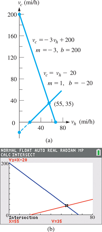
Fig. 5.19
We see that the point of intersection is (55, 35), which means that the solution is and Checking in the statement of the problem, we have
INCONSISTENT AND DEPENDENT SYSTEMS
The lines of each system in the previous examples intersect in a single point, and each system has one solution. Such systems are called consistent and independent. Most systems that we will encounter have just one solution. However, as we now show, not all systems have just one such solution. The following examples illustrate a system that has no solution and a system that has an unlimited number of solutions.
EXAMPLE 7 Inconsistent system
Solve the system of equations
Writing each of these equations in slope-intercept form, we have for the first equation
For the second equation, we have
From these, we see that each line has a slope of and that the y-intercepts are and Therefore, we know that the y-intercepts are different, but the slopes are the same. Because the slope indicates that each line rises unit for y for each unit x increases, the lines are parallel and do not intersect, as shown in Fig. 5.20.
NOTE
[This means that there are no solutions for this system of equations. Such a system is called inconsistent.]
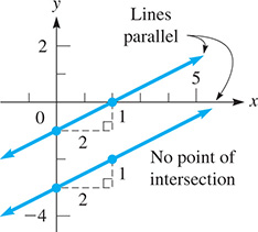
Fig. 5.20
EXAMPLE 8 Dependent system
Solve the system of equations
We find that the intercepts and a third point for the first line are (9, 0), and For the second line, we then find that the intercepts are the same as for the first line. We also find that the check point also satisfies the equation of the second line. This means that the two lines are really the same line.
Another check is to write each equation in slope-intercept form. This gives us the equation for each line. See Fig. 5.21.
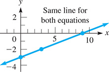
Fig. 5.21
NOTE
[Because the lines are the same, the coordinates of any point on this common line constitute a solution of the system. Since no unique solution can be determined, the system is called dependent.]
Later in the chapter, we will show algebraic ways of finding out whether a given system is consistent, inconsistent, or dependent.
EXERCISES 5.2
In Exercises 1–4, answer the given questions about the indicated examples of this section.
In Example 2, is a solution?
In the second equation of Example 4, if is replaced with what is the solution?
In Example 7, what changes occur if the 6 in the first equation is changed to a 2?
In Example 8, by changing what one number in the first equation does the system become (a) inconsistent? (b) consistent?
In Exercises 5–12, determine whether or not the given pair of values is a solution of the given system of linear equations.
In Exercises 13–28, solve each system of equations by sketching the graphs. Use the slope and the y-intercept or both intercepts. Estimate the result to the nearest 0.1 if necessary.
In Exercises 29–40, solve each system of equations to the nearest 0.001 for each variable by using a calculator.
In Exercises 41–44, solve the given problems.
In planning a search pattern from an aircraft carrier, a pilot plans to fly at p mi/h relative to a wind that is blowing at w mi/h. Traveling with the wind, the ground speed would be 300 mi/h, and against the wind the ground speed would be 220 mi/h. This leads to two equations:
Are the speeds 260 mi/h and 40 mi/h?
The electric resistance R of a certain resistor is a function of the temperature T given by the equation where a and b are constants. If when and when we can find the constants a and b by substituting and obtaining the equations
Are the constants and
The forces acting on part of a structure are shown in Fig. 5.22. An analysis of the forces leads to the equations

Fig. 5.22
Are the forces and
A student earned $4000 during the summer and decided to put half into an IRA (Individual Retirement Account). If the IRA was invested in two accounts earning 4.0% and 5.0%, the total income for the first year is $92. The equations to determine the amounts of x and y are
Are the amounts and
In Exercises 45–50, graphically solve the given problems. A calculator may be used.
Chains support a crate, as shown in Fig. 5.23. The equations relating tensions and are given below. Determine the tensions to the nearest 1 N from the graph.
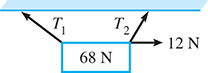
Fig. 5.23
An architect designing a parking lot has a row 202 ft wide to divide into spaces for compact cars and full-size cars. The architect determines that 16 compact car spaces and 6 full-size car spaces use the width, or that 12 compact car spaces and 9 full-size car spaces use all but 1 ft of the width. What are the widths (to the nearest 0.1 ft) of the spaces being planned? See Fig. 5.24.

Fig. 5.24
47. A small plane can fly 780 km with a tailwind in 3 h. If the tailwind is 50% stronger, it can fly 700 km in 2 h 30 min. Find the speed p of the plane in still air, and the speed w of the wind.
The equations relating the currents and shown in Fig. 5.25 are given below. Find the currents to the nearest 0.1 A.
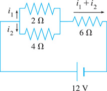
Fig. 5.25
A construction company placed two orders, at the same prices, with a lumber retailer. The first order was for 8 sheets of plywood and 40 framing studs for a total cost of $304. The second order was for 25 sheets of plywood and 12 framing studs for a total cost of $498. Find the price of one sheet of plywood and one framing stud.
A certain car gets 21 mi/gal in city driving and 28 mi/gal in highway driving. If 18 gal of gas are used in traveling 448 mi, how many miles were driven in the city, and how many were driven on the highway (assuming that only the given rates of usage were actually used)?
In Exercises 51–52, find the required values.
Determine the values of m and b that make the following system have no solution:
What, if any, value(s) of m and b result in the following system having (a) one solution, (b) an unlimited number of solutions?
Answer to Practice Exercises
Yes