Search in book...
Toggle Font Controls
Create new playlist

Name your new playlist

Playlist description (optional)
Sign In

Email address

Password

Forgot Password?

or

Continue with Facebook

Continue with Google
Sign Up

Full Name

Email address

Confirm Email Address

Password

or

Continue with Facebook

Continue with Google

13.1 Exponential Functions

The Exponential Function • Graphing Exponential Functions • Features of Exponential Functions

In Chapter 11, we showed that any rational number can be used as an exponent. Now letting the exponent be a variable, we define the exponential function as

y = b^{x}

$y = b^{x}$ (13.1)

where $b > 0, b \neq 1,$ $b > 0, b \neq 1,$ and x is any real number. The number b is called the base.

For an exponential function, we use only real numbers. Therefore, $b > 0,$ $b > 0,$ because if b were negative and x were a fractional exponent with an even-number denominator, y would be imaginary. Also, $b \neq 1,$ $b \neq 1,$ since 1 to any real power is 1 (y would be constant).

EXAMPLE 1 Exponential functions

From the definition, $y = 3^{x}$ $y = 3^{x}$ is an exponential function, but $y = {(- 3)}^{x}$ $y = {(- 3)}^{x}$ is not because the base is negative. However, $y = - 3^{x}$ $y = - 3^{x}$ is an exponential function, because it is $- 1$ $- 1$ times $3^{x},$ $3^{x},$ and any real-number multiple of an exponential function is also an exponential function.

Also, $y = {(\sqrt{3})}^{x}$ $y = {(\sqrt{3})}^{x}$ is an exponential function since it can be written as $y = 3^{x / 2} .$ $y = 3^{x / 2} .$ As long as x is a real number, so is x/2. Therefore, the exponent of 3 is real.

The function $y = 3^{- x}$ $y = 3^{- x}$ is an exponential function. If x is real, so is $- x .$ $- x .$

Other exponential functions are: $y = - 2 (8^{- 0.55 x})$ $y = - 2 (8^{- 0.55 x})$ and $y = 35 {(1.0001)}^{x} .$ $y = 35 {(1.0001)}^{x} .$

EXAMPLE 2 Evaluating an exponential function

Evaluate the function $y = - 2 (4^{x})$ $y = - 2 (4^{x})$ for the given values of x.

If $x = 2, y = - 2 (4^{2}) = - 2 (16) = - 32.$ $x = 2, y = - 2 (4^{2}) = - 2 (16) = - 32.$
If $x = - 2, y = - 2 (4^{- 2}) = - 2/16 = - 1/8.$ $x = - 2, y = - 2 (4^{- 2}) = - 2/16 = - 1/8.$
If $x = 3/2, y = - 2 (4^{3/2}) = - 2 (8) = - 16.$ $x = 3/2, y = - 2 (4^{3/2}) = - 2 (8) = - 16.$
If $x = \sqrt{2}, y = - 2 (4^{\sqrt{2}}) = - 14.206$ $x = \sqrt{2}, y = - 2 (4^{\sqrt{2}}) = - 14.206$ (calculator evaluation).
If $x = π, y = - 2 (4^{π}) = - 155.76$ $x = π, y = - 2 (4^{π}) = - 155.76$ (calculator evaluation).

GRAPHING EXPONENTIAL FUNCTIONS

We now show some representative graphs of the exponential function.

EXAMPLE 3 Graphing an exponential function

Plot the graph of $y = 2^{x} .$ $y = 2^{x} .$

For this function, we have the values in the following table:

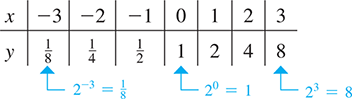
A table lists the corresponding values of x and y.

.1-2 Full Alternative Text

The curve is shown in Fig. 13.1(a). In Chapter 1, we used only integer exponents, and the enlarged points are for these values. In Chapter 11, we introduced rational exponents, and using them would fill in many points between those for integers, but all the points for irrational numbers would be missing and the curve would be dotted [see Fig. 13.1(b)]. Using all real numbers for exponents, including the irrational numbers, we have all points on the curve shown in Fig. 13.1(a).

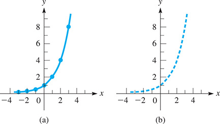
Two curves. Figure ay has a curve that rises from the negative x-axis and through (negative 3, one-eighth), (negative 2, one-fourth), (negative 1, one-half), (0, 1), (1, 2), (2, 4), and (4, 8). Figure b is the same curve in dot form. — Fig. 13.1

We see that the x-axis is an asymptote of the curve. The points on the left side of the graph get closer and closer to the x-axis, but they never touch it.

The bases b of the exponential function of greatest importance in applications are greater than 1. However, in order to understand how the exponential function differs somewhat if $b < 1,$ $b < 1,$ we now use a calculator to display such a graph.

EXAMPLE 4 Exponential function on a calculator

Display the graph of $y = 3 {(\frac{1}{2})}^{x}$ $y = 3 {(\frac{1}{2})}^{x}$ on a calculator.

For this function, ${(1/2)}^{x} = 1 / 2^{x} = 2^{- x} .$ ${(1/2)}^{x} = 1 / 2^{x} = 2^{- x} .$ Because x may be any real number, as x becomes more negative, y increases more rapidly. Therefore, on a calculator, we let $y_{1} = 3 {(1/2)}^{x} [{or y}_{1} = 3 ({.5}^{x})]$ $y_{1} = 3 {(1/2)}^{x} [{or y}_{1} = 3 ({.5}^{x})]$ and have the display in Fig. 13.2 with the window settings shown.

A curve falls through (0, 3), approaching the x-axis with decreasing steepness. The window is [negative 3, 3] by [negative 2, 24]. — Fig. 13.2

Any exponential curve where $b > 1$ $b > 1$ will be similar in shape to that shown in Fig. 13.1, and if $b < 1,$ $b < 1,$ it will be similar to the curve in Fig. 13.2. From these examples, we can see that exponential functions have the following basic features.

As we have noted, exponential functions are important in many applications. We now illustrate an application in the next example, and others are shown in the exercises.

EXAMPLE 5 Exponential function—rocket trajectory

A computer analysis of a rocket trajectory showed its height h (in m) as a function of time t (in s) was $h = 1600 (1 - e^{- 0.40 t}) .$ $h = 1600 (1 - e^{- 0.40 t}) .$ Display the graph of this function on a calculator. Here e is the number introduced on page 356 and is equal to approximately 2.718.

Here, $e^{- 0.40 t} = 1$ $e^{- 0.40 t} = 1$ for $t = 0,$ $t = 0,$ which means $h = 0$ $h = 0$ for $t = 0.$ $t = 0.$ Also, $e^{- 0.40 t}$ $e^{- 0.40 t}$ becomes smaller as t increases, and this means h cannot be greater than 1600 m. Therefore, $h = 1600 m$ $h = 1600 m$ is a horizontal asymptote. This leads to the settings and curve shown in Fig. 13.3. Here we have used y for h, x for t, and $y_{1} = 1600 (1 - e^{- .4 x}) .$ $y_{1} = 1600 (1 - e^{- .4 x}) .$

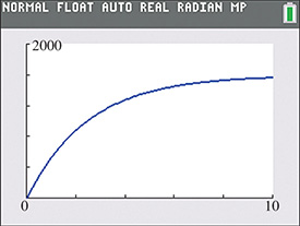
A curve begins at (0, 0), rising with decreasing steepness to (10, 1600). — Fig. 13.3

EXERCISES 13.1

In Exercises 1 and 2, perform the indicated operations if the given changes are made in the indicated examples of this section.

In Example 2(c), change the sign of x and then evaluate.
In Example 3, change the sign of the exponent and then plot the graph.

In Exercises 3–6, use a calculator to evaluate (to three significant digits) the given numbers.

$3^{\sqrt{5}}$ $3^{\sqrt{5}}$
${1.5}^{π}$ ${1.5}^{π}$
${(2 π)}^{- e}$ ${(2 π)}^{- e}$
${(2 e)}^{- \sqrt{2}}$ ${(2 e)}^{- \sqrt{2}}$

In Exercises 7–10, determine if the given functions are exponential functions.

1. $y = 5^{x}$ $y = 5^{x}$
2. $y = 5^{- x}$ $y = 5^{- x}$
1. $y = - 7^{x}$ $y = - 7^{x}$
2. $y = {(- 7)}^{- x}$ $y = {(- 7)}^{- x}$
1. $y = - 7 {(- 5)}^{- x}$ $y = - 7 {(- 5)}^{- x}$
2. $y = - 7 (5^{- x})$ $y = - 7 (5^{- x})$
1. $y = {(\sqrt{5})}^{- x}$ $y = {(\sqrt{5})}^{- x}$
2. $y = - {(\sqrt{- 5})}^{x}$ $y = - {(\sqrt{- 5})}^{x}$

In Exercises 11–16, evaluate the exponential function

y = 4^{x}

$y = 4^{x}$ for the given values of x.

$x = 0.5$ $x = 0.5$
$x = 4$ $x = 4$
$x = - 2$ $x = - 2$
$x = - 0.5$ $x = - 0.5$
$x = - 3/2$ $x = - 3/2$
$x = 5/2$ $x = 5/2$

In Exercises 17–22, plot the graphs of the given functions.

$y = 4^{x}$ $y = 4^{x}$
$y = {0.25}^{x}$ $y = {0.25}^{x}$
$y = 0.2 (10^{- x})$ $y = 0.2 (10^{- x})$
$y = - 5 ({1.6}^{- x})$ $y = - 5 ({1.6}^{- x})$
$y = 0.5 π^{x}$ $y = 0.5 π^{x}$
$y = 2 e^{x}$ $y = 2 e^{x}$

In Exercises 23–30, display the graphs of the given functions on a calculator.

$y = 0.3 {(2.55)}^{x}$ $y = 0.3 {(2.55)}^{x}$
$y = - 1.5 {(4.15)}^{x}$ $y = - 1.5 {(4.15)}^{x}$
$y = 0.1 ({0.25}^{2 x})$ $y = 0.1 ({0.25}^{2 x})$
$y = 0.4 {(0.95)}^{3 x}$ $y = 0.4 {(0.95)}^{3 x}$
$i = 1.2 (2 + 6^{- t})$ $i = 1.2 (2 + 6^{- t})$
$y = 0.5 e^{- x}$ $y = 0.5 e^{- x}$
1. $y = 10^{x}$ $y = 10^{x}$
2. $y = 2^{x}$ $y = 2^{x}$
3. $y = {1.1}^{x}$ $y = {1.1}^{x}$
1. $y = {0.1}^{x}$ $y = {0.1}^{x}$
2. $y = {0.5}^{x}$ $y = {0.5}^{x}$
3. $y = {0.9}^{x}$ $y = {0.9}^{x}$

In Exercises 31–46, solve the given problems.

Find the base b of the function $y = b^{x}$ $y = b^{x}$ if its graph passes through the point (3, 64).
Find the base b of the function $y = b^{x}$ $y = b^{x}$ if its graph passes through the point $(- 2, 64) .$ $(- 2, 64) .$
For the function $f (x) = b^{x},$ $f (x) = b^{x},$ show that $f (c + d) = f (c) \cdot f (d) .$ $f (c + d) = f (c) \cdot f (d) .$
For the function $f (x) = b^{x},$ $f (x) = b^{x},$ show that $f (c - d) = f (c) / f (d) .$ $f (c - d) = f (c) / f (d) .$
Use a calculator to graph the function $y = 2^{| x |} .$ $y = 2^{| x |} .$
To show the damping effect of an exponential function, use a calculator to display the graph of $y = (x^{3}) (2^{- x}) .$ $y = (x^{3}) (2^{- x}) .$ Be sure to use appropriate window settings.
Use a calculator to find the value(s) for which $x^{2} = 2^{x} .$ $x^{2} = 2^{x} .$
Use a calculator to find the value(s) for which $x^{3} = 3^{x} .$ $x^{3} = 3^{x} .$
For $f (x) = A e^{k x},$ $f (x) = A e^{k x},$ find the expression for $\frac{f (x + 1) - f (x)}{f (x)} .$ $\frac{f (x + 1) - f (x)}{f (x)} .$
A medical research lab is growing a virus for a vaccine that grows at a rate of 2.3% per hour. If there are 500.0 units of the virus originally, the amount present after t hours is given by $N = 500.0 {(1.023)}^{t} .$ $N = 500.0 {(1.023)}^{t} .$ How many units of the virus are present after two days?
The value V of a bank account in which $250 is invested at 5.00% interest, compounded annually, is $V = 250 {(1.0500)}^{t},$ $V = 250 {(1.0500)}^{t},$ where t is the time in years. Find the value of the account after 4 years.
The intensity I of an earthquake is given by $I = I_{0} {(10)}^{R},$ $I = I_{0} {(10)}^{R},$ where $I_{0}$ $I_{0}$ is a minimum intensity for comparison and R is the Richter scale magnitude of the earthquake. Evaluate I in terms of $I_{0}$ $I_{0}$ if $R = 5.5.$ $R = 5.5.$

Fig. 13.4
The electric current i (in mA) in the circuit shown in Fig. 13.4 is $i = 2.5 (1 - e^{- 0.10 t}),$ $i = 2.5 (1 - e^{- 0.10 t}),$ where t is the time (in s). Evaluate i for $t = 5.0 ms (1 ms = 10^{- 3} s) .$ $t = 5.0 ms (1 ms = 10^{- 3} s) .$
The strength I of a certain cable signal is given by $I = I_{0} e^{- 0.0015 x},$ $I = I_{0} e^{- 0.0015 x},$ where $I_{0}$ $I_{0}$ is the signal strength at the source and x is the distance (in km) from the source. What percent of the signal strength is lost 15 km from the source?
The flash unit on a camera operates by releasing the stored charge on a capacitor. For a particular unit, the charge q (in $μ C$ $μ C$ ) as a function of the time t (in s) is $q = 100 e^{- 10 t} .$ $q = 100 e^{- 10 t} .$ Display the graph on a calculator.
The height y (in m) of the Gateway Arch in St. Louis (see Fig. 13.5) is given by $y = 230.9 - 19.5 (e^{x / 38.9} + e^{- x / 38.9}),$ $y = 230.9 - 19.5 (e^{x / 38.9} + e^{- x / 38.9}),$ where x is the distance (in m) from the point on the ground level directly below the top. Display the graph on a calculator.

Fig. 13.5

Answers to Practice Exercises

..................Content has been hidden....................

You can't read the all page of ebook, please click here login for view all page.

Table of Contents for 13.1 Exponential Functions

Create new playlist

Sign In

Sign Up

Table of Contents for
13.1 Exponential Functions