15.2 The Roots of an Equation
The Fundamental Theorem of Algebra • Linear Factors • Complex Roots • Remaining Quadratic Factor
In this section, we present certain theorems that are useful in determining the number of roots in the equation and the nature of some of these roots. In dealing with polynomial equations of higher degree, it is helpful to have as much of this kind of information as we can find before actually solving for all of the roots, including any possible complex roots. A graph does not show the complex roots an equation may have, but we can verify the real roots, as we show by use of a graphing calculator in some of the examples that follow.
The first of these theorems is so important that it is called the fundamental theorem of algebra. It states:
Every polynomial equation has at least one (real or complex) root.
The proof of this theorem is of an advanced nature, and therefore we accept its validity at this time. However, using the fundamental theorem, we can show the validity of other theorems that are useful in solving equations.
Let us now assume that we have a polynomial equation and that we are looking for its roots. By the fundamental theorem, we know that it has at least one root. Assuming that we can find this root by some means (the factor theorem, for example), we call this root Thus,
where is the polynomial quotient found by dividing f(x) by However, because the fundamental theorem states that any polynomial equation has at least one root, this must apply to as well. Let us assume that has the root Therefore, this means that Continuing this process until one of the quotients is a constant a, we have
Note that one linear factor appears each time a root is found and that the degree of the quotient is one less each time. Thus, there are n linear factors, if the degree of f(x) is n.
Therefore, based on the fundamental theorem of algebra, we have the following two related theorems.
These theorems are illustrated in the following example.
EXAMPLE 1 Illustrating fundamental theorem
For the function we are given the factors that we show. In the next section, we will see how to find these factors.
For the function f(x), we have
Therefore,
The degree of f(x) is 4. There are four linear factors: and There are four roots of the equation: 3, 1, and Thus, we have verified each of the theorems above for this example.
It is not necessary for each root of an equation to be different from the other roots. Actually, there is no limit as to the number of roots an equation can have that are the same. For example, the equation has sixteen roots, all of which are 1. Such roots are referred to as multiple (or repeated) roots. In this case, the root of 1 has a multiplicity of 16.
When we solve the equation the roots are j and In fact, for any equation (with real coefficients) that has a root of the form there is also a root of the form This is summarized below.
EXAMPLE 2 Illustrating complex roots
Consider the equation
The factor shows that there is a triple root of 1, and there is a total of five roots, because the highest-power term would be if we were to multiply out the function. To find the other two roots, we use the quadratic formula on the factor This is permissible, because we are finding the values of x for
For this, we have
Thus,
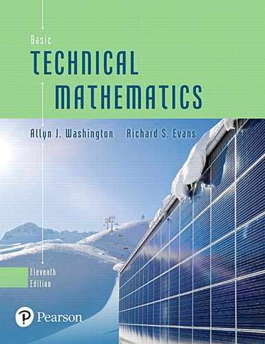
Therefore, the roots of are and In the graph of f(x) shown in Fig. 15.1, the zero feature gives a value of but the calculator display does not show that it is a triple root, or that there are complex roots.

Fig. 15.1
NOTE
[From Example 2, we can see that whenever enough roots are known so that the remaining factor is quadratic, it is possible to find the remaining roots from the quadratic formula.]
This is true for finding real or complex roots.
EXAMPLE 3 Solving equation—given one root
Solve the equation is a root.
Using synthetic division and the given root, we have the setup shown at the left. From this, we see that
We know that is a factor from the given root and that is a factor found from synthetic division. This second factor can be factored as
Therefore, we have
This means the roots are and 2. Because the three roots are real, they can be found from a calculator display, as shown in Fig. 15.2.
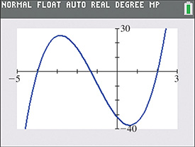
Fig. 15.2
EXAMPLE 4 Solving equation—given two roots
Solve and 2 are roots.
Using synthetic division and the root the first setup at the left shows that
We now know that must be a factor of because it is a factor of the original function. Again, using synthetic division and this time the root 2, we have the second setup at the left. Thus,
Because the original equation can now be written as
the remaining two roots are found by solving
by the quadratic formula. This gives us
Therefore, the roots are and
EXAMPLE 5 Solving equation—given double root
Solve the equation given that 2 is a double root.
Using synthetic division, we have the first setup at the left. It tells us that
Also, because 2 is a double root, it must be a root of Using synthetic division again, we have the second setup at the left. This second quotient factors into The roots are 2, 2, and 5.
NOTE
[Because the quotient of the first division is the dividend for the second division, both divisions can be done without rewriting the first quotient as follows:]

EXAMPLE 6 Solving equation—given complex root
Solve the equation given that is a root.
Because is a root, we know that is also a root. Using synthetic division twice, we can then reduce the remaining factor to a quadratic function.
The quadratic factor factors into Therefore, the roots of the equation are and As we can see, the calculator display in Fig. 15.3 shows only the real roots.

Fig. 15.3
GRAPHICAL FEATURES INDICATING NUMBER AND TYPES OF ROOTS
If f(x) is of degree n and the roots of are real and different, the graph of f(x) crosses the x-axis n times and f(x) changes signs as it crosses. See Fig. 15.4, where the equation has four changes of sign, and the graph crosses four times.
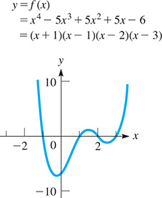
Fig. 15.4
For each pair of complex roots, the number of times the graph crosses the x-axis is reduced by two (Fig. 15.5). For multiple roots, the graph crosses the x-axis once if the multiple is odd, or is tangent to the x-axis if the multiple is even (Fig. 15.6).
Fig. 15.5
The graph must cross the x-axis at least once if the degree of f(x) is odd, because the range includes all real numbers (Figs. 15.5 and 15.6). The curve may not cross the x-axis if the degree of f(x) is even, because the range is bounded at a minimum point or a maximum point (Fig. 15.7), as we have seen for a quadratic function.
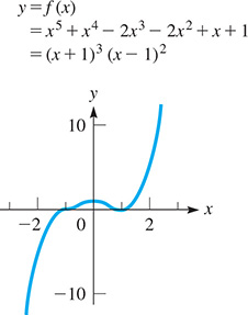
Fig. 15.6

Fig. 15.7
EXERCISES 15.2
In Exercises 1 and 2, make the given changes in the indicated examples of this section and then solve the resulting equation.
In Example 2, change the middle term of the second factor to 2x.
In Example 6, change the middle three terms to the left of the given the same root.
In Exercises 3–6, find the roots of the given equations by inspection.
In Exercises 7–26, find the remaining roots of the given equations using synthetic division, given the roots indicated.
(5 is a double root)
( is a double root)
(1 is a triple root)
( is a double root; 2j is a root)
(j is a double root)
In Exercises 27 and 28, answer the given questions.
 Why cannot a third-degree polynomial function with real coefficients have zeros of 1, 2, and j?
- How can the graph of a fourth-degree polynomial equation have its only x-intercepts as 0, 1, and 2?
In Exercises 29–32, solve the given problems.
Find k such that is a factor of
Find k such that is a factor of
Equations of the form are called elliptic curves and are used in cryptography. If for the curve use synthetic division to show that one possible value of x is Then find any other possible values of x.
Form a polynomial equation of the smallest possible degree and with integer coefficients, having a double root of 3, and a root of j.