
22.7 Nonlinear Regression
Nonlinear Regression • Types of Curves on a Calculator • Choosing an Appropriate Regression Model
The method of least-squares regression can be extended to cases where the data points tend to curve rather than follow a straight line. This is called nonlinear regression. The specific mathematical techniques and formulas used for nonlinear regression are beyond the scope of this chapter. However, a calculator can be used to find many different kinds of nonlinear regression models. Figure 22.27 lists the types of regression available on most graphing calculators along with some examples of their shapes.
NOTE
[To choose an appropriate model, one should first plot the data to get a scatterplot. Then, depending on the shape of the points, an appropriate model can be chosen.]

Fig. 22.27
When more than one type of model seems reasonable, we can try different types to see which one fits best. In nonlinear regression, the calculator still provides values of r, or . Although these are not calculated using the same formulas as in linear regression, they still measure how well the regression model fits the data points. As before, values close to 1 (or for r) indicate a good fit. The following examples illustrate the process of choosing and determining a regression model.
NOTE
[Practical considerations should also be taken into account when choosing a model. For example, if it is known that a quantity will continually decrease, one should try to avoid choosing a model that would eventually predict increases.]
EXAMPLE 1 Choosing a regression model—volume and pressure of a gas
In a physics experiment, the pressure P and volume V of a gas were measured at constant temperature. The resulting data are shown in the table below and plotted on a calculator in Fig. 22.28.
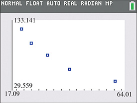
Fig. 22.28
| Volume, | 21.0 | 25.0 | 31.8 | 41.1 | 60.1 |
| Pressure, P (kPa) | 120.0 | 99.2 | 81.3 | 60.6 | 42.7 |
Based on the curved downward trend of the points, the types of regression models that are reasonable to try here are logarithmic, exponential, and power. After trying all three, the power regression model clearly fits the data the best. The power regression equation is as shown in Fig. 22.29(a). The graph of the model through the scatterplot is shown in Fig. 22.29(b). The fact that r is close to –1 and is close to 1 indicate the model fits the data very well.
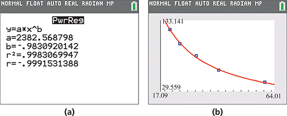
Fig. 22.29
Graphing calculator screenshots: goo.gl/GZYkRH
Using the variables in our problem, we can rewrite the regression equation as . This can be used to predict either variable when given the other. For example, to predict the pressure when the volume is we get (interpolation).
EXAMPLE 2 Choosing a regression model—bacteria growth
In a medical research lab, an experiment was performed to measure the number N of bacteria present t min after the start of the experiment. The following table shows the resulting data, and the scatterplot is shown in Fig. 22.30.
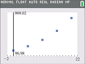
Fig. 22.30
| Time, t (min) | 0 | 5 | 10 | 15 | 20 |
| Number of bacteria, N | 200 | 282 | 398 | 568 | 806 |
Because of the curved upward trend of the points, we will try both a quadratic and an exponential regression model. The results from a calculator are shown in Figs. 22.31 and 22.32. Both models provide a very good fit of the data points.
Quadratic regression model

Fig. 22.31
Graphing calculator screenshots: bit.ly/
Exponential regression model
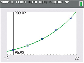
Fig. 22.32
Graphing calculator screenshots: bit.ly/
Because both models fit the data well, either can be used. However, since it is known that bacteria grow exponentially, the exponential model will likely fit better in the long run. Suppose we wish to estimate the number of bacteria present after 25 min. Using the exponential model, we have (extrapolation).
EXERCISES 22.7
In Exercises 1–12, use a calculator to find a regression model for the given data. Graph the scatterplot and regression model on the calculator. Use the regression model to make the indicated predictions.
Find an exponential regression model for the given data:
x 0 10 20 30 40 y 350 570 929 1513 2464 Find a logarithmic regression model for the given data:
x 1 4 8 12 16 y 2 9 11 14 15 The following data show the tensile strength (in ) of brass (a copper-zinc alloy) that contains different percents of zinc.
Percent of Zinc 0 5 10 15 20 30 Tensile Strength 0.32 0.36 0.39 0.41 0.44 0.47 Find a logistic regression model for the data. Predict the tensile strength of brass that contains 25% zinc.
The following data were found for the distance y that an object rolled down an inclined plane in time t. Find a quadratic regression model for these data. Predict the distance at 2.5 s.
t (s) 1.0 2.0 3.0 4.0 5.0 y (cm) 6.0 23 55 98 148 The increase in length y of a certain metallic rod was measured in relation to particular increases x in temperature. Find a quadratic regression model for the given data.
x 50.0 100 150 200 250 y (cm) 1.00 4.40 9.40 16.4 24.0 The pressure p at which Freon, a refrigerant, vaporizes for temperature T is given in the following table. Find a quadratic regression model. Predict the vaporization pressure at .
T (° F) 0 20 40 60 80 23 35 49 68 88 A fraction f of annual hot-water loads at a certain facility are heated by solar energy. The fractions f for certain values of the collector area A are given in the following table. Find a power regression model for these data.
0 12 27 56 90 f 0.0 0.2 0.4 0.6 0.8 The output torque (in J) of a certain engine was measured at various frequencies (in r/min) with the following results. Find a power regression model for these data. Predict the output torque for a frequency of 3500 r/min. Is this interpolation or extrapolation?
f (r/min) 500 1000 1500 2000 2500 3000 T (J) 220 102 77 50 43 30 The resonant frequency f of an electric circuit containing a capacitor was measured as a function of the inductance L in the circuit. The following data were found. Find a power regression model for these data.
L (H) 1.0 2.0 4.0 6.0 9.0 f (Hz) 490 360 250 200 170 The displacement y of an object at the end of a spring at given times t is shown in the following table. Find an exponential regression model for this. Predict the displacement at 2.5 s. Is this interpolation or extrapolation?
t (s) 0.0 0.5 1.0 1.5 2.0 3.0 y (cm) 6.1 3.8 2.3 1.3 0.7 0.3 The average daily temperatures T (in ) for each month in Minneapolis (National Weather Service records) are given in the following table. ( etc.).
Month, t 1 2 3 4 5 6 7 8 9 10 11 12 T 11 18 29 46 57 68 73 71 61 50 33 19 Find a sinusoidal regression model for these data.