16.5 Gaussian Elimination
Row Echelon Form • Gaussian Elimination • Number of Possible Solutions • Consistent and Inconsistent Systems
We now show a general method that can be used to solve a system of linear equations. The procedure used in this method is similar to that used in finding the inverse of a matrix in Section 16.3. It is known as Gaussian elimination, and as noted in the chapter introduction, it was developed in the early 1800s by Karl Gauss. Today, it is commonly used in computer programs for the solutions of systems of linear equations.
When using this method, we use certain row operations to convert the system of equations to row echelon form. Then the solution can be found by substituting back into the equations from the bottom up. The following examples illustrate this method.
EXAMPLE 1 Row echelon form
The system of equations to the left is said to be in row echelon form. We see that the third equation directly gives us the value Since the second equation contains only y and z, we can now substitute into the second equation to get Then we can find x by substituting and into the first equation, and get Therefore, after writing the system of equations in the form to the left, the solution is completed by substituting back, starting with the last equation.
The method of Gaussian elimination is based on first rewriting the given system of equations in row echelon form like in Example 1, so that the last equation shows the value of one of the unknowns, and the others are found by substituting back. The method to obtain the proper form is based on the use of any of the following three operations on the equations of the original system of equations.
Using three linear equations in three unknowns as an example, by using the above operations, we can change the system
into the equivalent system in row echelon form
The solution is completed by substituting the value of z into the second equation, and then substituting the values of y and z into the first equation, as in Example 1.
EXAMPLE 2 Gaussian elimination with two equations
Solve the following system of equations using Gaussian elimination:
The steps are given below, with the necessary row operations shown in red:
To find the value of x, we substitute into the first equation: or
Thus, the solution is which checks when substituted into the original equations.
EXAMPLE 3 Gaussian elimination with three equations
Solve the following system of equations using Gaussian elimination:
In this example, we will perform the row operations on the augmented matrix, which includes the coefficients and constant terms, but not the variables. The equal signs are replaced with dotted lines. The steps are shown below.
The last line above shows that This can be substituted into the second equation to find y, and then the values of x and y can be substituted into the first equation to find x.
Thus, the solution is This solution checks in the original equations.
Note that in this example, it is possible to continue performing row operations until the left side of the augmented matrix is the identity matrix. This is called reduced row echelon form (rref). In this form, the system is completely solved and there is no need to back-substitute from the bottom up. Many calculators have a rref feature that can be used to solve systems of equations (see Example 3 in Section 5.5). Figure 16.16 shows the calculator solution for this example.
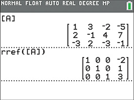
Fig. 16.16
Graphing calculator keystrokes: bit.ly/
EXAMPLE 4 Gaussian elimination leading to infinite solutions
Solve the following system of equations using Gaussian elimination:
We will again work with the augmented matrix. Since the first equation doesn’t contain x, we start by interchanging the first two equations. The steps are shown below.
The last row of zeros indicates that z can be any number. But it is still possible to express both x and y in terms of z. We first solve the equation in the second row for y in terms of z, which results in Then this expression can be substituted into the equation in the top row to solve for x in terms of z.
Therefore, the solution is given by and where z can be any number.
NOTE
[This means there are an infinite number of solutions.]
For example, if then and
NOTE
[Note that the original matrix of coefficients on the left of the dotted line has a determinant of zero, and therefore its inverse does not exist. Thus, the method described in Section 16.4 cannot be used to solve this system. This underscores the importance of Gaussian elimination.]
POSSIBLE NUMBER OF SOLUTIONS
When we solved systems of linear equations in Chapter 5, we found that not all systems have unique solutions, as they do in Examples 2 and 3. In Example 4, we illustrated the use of Gaussian elimination on a system of equations for which the solution is not unique.
In Example 4, one of the equations became and there was an unlimited number of solutions. If any of the equations of a system becomes then the system is inconsistent and there is no solution. Example 5 illustrates such a system.
If a system has more unknowns than equations, or it can be written this way, as in Example 4, it usually has an unlimited number of solutions. It is possible, however, that such a system is inconsistent.
If a system has more equations than unknowns, it is inconsistent unless enough equations become such that at least one solution is found. The following example illustrates two systems in which there are more equations than unknowns.
EXAMPLE 5 Consistent and inconsistent systems
Solve the following systems of equations by Gaussian elimination.
The solutions are shown at the left. We note that each system has three equations and two unknowns.
In the solution of the first system, the third equation becomes and only two equations are needed to find the solution
In the solution of the second system, the third equation becomes which means the system is inconsistent and there is no solution.
Graphing the systems, note that in Fig. 16.17, each of the lines passes through the point (1, 2), whereas in Fig. 16.18, there is no point common to the three lines.

Fig. 16.17
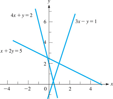
Fig. 16.18
EXERCISES 16.5
In Exercises 1 and 2, make the given changes in the indicated examples of this section, and then solve the resulting systems using Gaussian elimination.
In Example 2, interchange the two equations and then solve the system with the equations in this order.
In Example 5, change the third equation of the second system to
In Exercises 3–24, solve the given systems of equations by Gaussian elimination. If there is an unlimited number of solutions, find two of them.
In Exercises 25–28, solve the given system of equations by using the rref feature on a calculator.
In Exercises 29 and 30, solve the given problems using Gaussian elimination.
Solve the system and show that the result is the same as that obtained using Cramer’s rule as in Section 5.4. See page 160.
Solve the system and show that the solution depends on the value of a. What value of a does the solution show may not be used?
In Exercises 31–34, set up systems of equations and solve by Gaussian elimination.
Two jets are 2370 km apart and traveling toward each other, one at 720 km/h and the other at 860 km/h. How far does each travel before they pass?
The voltage across an electric resistor equals the current (in A) times the resistance (in ). If a current of 3.00 A passes through each of two resistors, the sum of the voltages is 10.5 V. If 2.00 A passes through the first resistor and 4.00 A passes through the second resistor, the sum of the voltages is 13.0 V. Find the resistances.
Three machines together produce 650 parts each hour. Twice the production of the second machine is 10 parts/h more than the sum of the production of the other two machines. If the first operates for 3.00 h and the others operate for 2.00 h, 1550 parts are produced. Find the production rate of each machine.
A business bought three types of computer programs to be used in offices at different locations. The first costs $35 each and uses 190 MB of memory; the second costs $50 each and uses 225 MB of memory; and the third costs $60 each and uses 130 MB of memory. If as many of the third type were purchased as the other two combined, with a total cost of $2600 and total memory requirement of 8525 MB, how many of each were purchased?