3.5 Graphs on the Graphing Calculator
Calculator Setup for Graphing • Solving Equations Graphically • Finding the Maximum or Minimum from a Graph • Shifting a Graph
In this section, we will see that a graphing calculator can display a graph quickly and easily. As we have pointed out, to use your calculator effectively, you must know the sequence of keys for any operation you intend to use. The manual for any particular model should be used for a detailed coverage of its features.
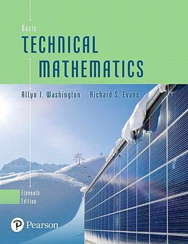
EXAMPLE 1 Entering the function: window settings
To graph the function first display then enter the The display for this is shown in Fig. 3.28(a).
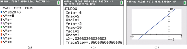
Fig. 3.28
Next use the window (or range) feature to set the part of the domain and the range that will be seen in the viewing window. For this function, set
in order to get a good view of the graph. The display for the window settings is shown in Fig. 3.28(b).
Then display the graph, using the graph (or exe) key. The display showing the graph of is shown in Fig. 3.28(c).
In Example 1, we noted that the window feature sets the intervals of the domain and range of the function that are seen in the viewing window. Unless the settings are appropriate, you may not get a good view of the graph.
EXAMPLE 2 Choose window settings carefully
In Example 1, the window settings were chosen to give a good view of the graph of However, if we had chosen settings of and we would get the view shown in Fig. 3.29. We see that very little of the graph can be seen. With some settings, it is possible that no part of the graph can be seen. Therefore, it is necessary to be careful in choosing the settings. This includes the scale settings (Xscl and Yscl), which should be chosen so that several (not too many or too few) axis markers are used.
![A calculator screen with a window that is [negative 3, 3] by [negative 3, 3]. Part of a smooth curve is visible in quadrant 2.](http://imgdetail.ebookreading.net/202009/01/9780136747826/9780136747826__basic-technical-mathematics__9780136747826__images__Fig03-29.jpg)
Fig. 3.29
Because the settings are easily changed, to get the general location of the graph, it is usually best to first choose intervals between the min and max values that are greater than is probably necessary. They can be reduced as needed.
Also, note that the calculator makes the graph just as we have been doing—by plotting points (square dots called pixels). It just does it a lot faster.
SOLVING EQUATIONS GRAPHICALLY
An equation can be solved by use of a graph. Most of the time, the solution will be approximate, but with a graphing calculator, it is possible to get good accuracy in the result. The procedure used is as follows:
EXAMPLE 3 Solving an equation graphically
Using a calculator, graphically solve the equation
Following the above procedure, we first rewrite the equation as and then set Next, we graph this function as shown in Fig. 3.30(a). Since the graph crosses the x-axis twice, the equation has two solutions which appear to be approximately and
Fig. 3.30
A graphing calculator can be used to find the x-intercepts with a high level of accuracy by using the zero feature. When using the zero feature, one must move the crosshairs on the calculator screen to choose a left bound (to the left of the x-intercept), a right bound (to the right of the x-intercept), and then a guess (near the x-intercept), pressing Enter after each entry. The calculator will then display the x-intercept. This process must be repeated twice, once for each x-intercept. The solutions, which are shown in Fig. 3.30(b) and (c), are and (rounded to the nearest thousandth). Note that these solutions are close to our original estimates.
EXAMPLE 4 Solving graphically—container dimensions
A rectangular container whose volume is is made with a square base and a height that is 2.00 cm less than the length of the side of the base. Find the dimensions of the container by first setting up the necessary equation and then solving it graphically on a calculator.
Let length of the side of the square base (see Fig. 3.31); the height is then This means the volume is or Because the volume is we have the equation

Fig. 3.31
To solve it graphically on a calculator, first rewrite the equation as and then set The calculator view is shown in Fig. 3.32, where we use only positive values of x, because negative values have no meaning. Using the zero feature, we find that is the approximate solution. Therefore, the dimensions are 3.94 cm, 3.94 cm, and 1.94 cm. Checking, these dimensions give a volume of The slight difference of is due to rounding off. A better check can be made by using the calculator value before rounding off. However, the final dimensions should be given only to three significant digits.

Fig. 3.32
EXAMPLE 5 Solving graphically—fuel cell power
The electric power P (in W) delivered by a certain fuel cell as a function of the resistance R (in ) in the circuit is given by Find (a) the maximum power, (b) the resistances that deliver a power of 40 W, and (c) the domain and range of the function.
By using the maximum feature on a calculator (and selecting a left bound, a right bound, and a guess), the maximum power is found to be 50 W as shown in Fig. 3.33. This occurs when
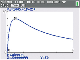
Fig. 3.33
To find the resistances that deliver 40 W of power, we can find the points of intersection between the given function and the function By using the intersect feature on a calculator (and choosing the first curve, the second curve, and a guess), the resistances are found to be and to the nearest hundredth. Note that the intersect feature must be applied twice, once for each intersecting point. See Fig. 3.34(a) and (b).

Fig. 3.34
Since it is not reasonable for the resistance to be negative, the domain consists of all values Since the power cannot be negative and the maximum power is 50 W, the range is all values
SHIFTING A GRAPH
By adding a positive constant to the right side of the function the graph of the function is shifted straight up. If a negative constant is added to the right side of the function, the graph is shifted straight down.
EXAMPLE 6 Shifting a graph vertically
If we add 2 to the right side of we get This will shift the graph of up 2 units.
If we add to the right side of we get This will shift the graph of down 3 units. Figure 3.35 shows the original function (in blue) along with both vertical shifts.
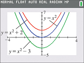
Fig. 3.35
By adding a constant to x in the function the graph of the function is shifted to the right or to the left.
CAUTION
Adding a positive constant to x shifts the graph to the left, and adding a negative constant to x shifts the graph to the right.
EXAMPLE 7 Shifting a graph horizontally
For the function if we add 2 to x, we get or if we add to x, we get The graphs of these three functions are displayed in Fig. 3.36.
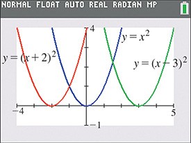
Fig. 3.36
We see that the graph of is 2 units to the left of and that the graph of is 3 units to the right of
Be very careful when shifting graphs horizontally. To check the direction and magnitude of a horizontal shift, find the value of x that makes the expression in parentheses equal to 0. For example, in Example 7, is 3 units to the right of because makes equal to zero. The point (3, 0) on is equivalent to the point (0, 0) on In the same way for and the graph of is shifted 2 units to the left of
Summarizing how a graph is shifted, we have the following:
EXAMPLE 8 Shifting vertically and horizontally
The graph of a function can be shifted both vertically and horizontally. To shift the graph of to the right 3 units and down 2 units, add to x and add to the resulting function. In this way, we get The graph of this function and the graph of are shown in Fig. 3.37.

Fig. 3.37
Note that the point on the graph of is equivalent to the point (0, 0) on the graph of Checking, by setting we get This means the graph of has been shifted 3 units to the right. The vertical shift of is clear.
EXERCISES 3.5
In Exercises 1 and 2, make the indicated changes in the given examples of this section and then solve.
In Example 3, change the sign on the left side of the equation from to
In Example 8, in the second line, change “to the right 3 units and down 2 units” to “to the left 2 units and down 3 units.”
In Exercises 3–18, display the graphs of the given functions on a graphing calculator. Use appropriate window settings.
In Exercises 19–28, use a graphing calculator to solve the given equations to the nearest 0.001.
In Exercises 29–40, use a graphing calculator to find the range of the given functions. Use the maximum or minimum feature when needed.
In Exercises 41–48, a function and how it is to be shifted is given. Find the shifted function, and then display the given function and the shifted function on the same screen of a graphing calculator.
up 1
down 2
right 3
left 4
down 3, left 2
up 4, right 3
up 1, left 1
down 2, right 2
In Exercises 49–52, use the function for which the graph is shown in Fig. 3.38 to sketch graphs of the indicated functions.
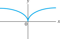
Fig. 3.38
In Exercises 53–60, solve the indicated equations graphically. Assume all data are accurate to two significant digits unless greater accuracy is given.
In an electric circuit, the current i (in A) as a function of voltage v is given by Find v for
For tax purposes, a corporation assumes that one of its computer systems depreciates according to the equation where V is the value (in dollars) after t years. According to this formula, when will the computer be fully depreciated (no value)?
Two cubical coolers together hold If the inside edge of one is 5.00 cm greater than the inside edge of the other, what is the inside edge of each?
The height h (in ft) of a rocket as a function of time t (in s) of flight is given by Determine when the rocket is at ground level. Also find the maximum height.
The length of a rectangular solar panel is 12 cm more than its width. If its area is find its dimensions.
A computer model shows that the cost (in dollars) to remove x percent of a pollutant from a lake is What percent can be removed for $25,000?
In finding the illumination at a point x feet from one of two light sources that are 100 ft apart, it is necessary to solve the equation Find x.
A rectangular storage bin is to be made from a rectangular piece of sheet metal 12 in. by 10 in., by cutting out equal corners of side x and bending up the sides. See Fig. 3.39. Find x if the storage bin is to hold

Fig. 3.39
In Exercises 61–68, solve the given problems.
The concentration C (in mg/L) of a drug in a patient’s bloodstream t hours after taking a pill is given by The patient should receive a second dose after the concentration has dropped below 1.50 mg/L. How long will this take?
The cutting speed s (in ft/min) of a saw in cutting a particular type of metal piece is given by where t is the time in seconds. What is the maximum cutting speed in this operation (to two significant digits)? (Hint: Find the range.)
 Referring to Exercise 60, explain how to determine the maximum possible capacity for a storage bin constructed in this way. What is the maximum possible capacity (to three significant digits)?
A balloon is being blown up at a constant rate. (a) Sketch a reasonable graph of the radius of the balloon as a function of time. (b) Compare to a typical situation that can be described by where r is the radius (in cm) and t is the time (in s).
A hot-water faucet is turned on. (a) Sketch a reasonable graph of the water temperature as a function of time. (b) Compare to a typical situation described by where T is the water temperature (in ) and t is the time (in s).
- Display the graph of with and with Describe the effect of the value of c.
- Display the graph of with and with Describe the effect of the value of c.
Answers to Practice Exercises
x: to 3: y: to 8 is a good window setting.
5 units down
2 units left, 3 units up