22.6 Linear Regression
Regression • Linear Regression • Method of Least Squares • Deviation • Least-squares Line • Using a Calculator • Interpolation • Extrapolation • Interpreting r and
In the previous sections of this chapter, we have discussed various statistical methods for graphically and numerically summarizing the values of a single variable. In this section, we will show how to describe the relationship between two different quantitative variables, which allows us to predict the value of one from the other. There are many situations where data points from paired data form a general straight-line pattern but don’t line up exactly along a straight line. In these cases, we wish to find the equation of a line that best fits the data points. The process of finding such a line is called linear regression.
In Chapters 5 and 21, we showed how the calculator can be used to find the equation of a regression line. In this section, we will show the mathematics behind the creation of this line and also discuss how to measure the strength of the linear relationship. We consider nonlinear regression in the next section.
EXAMPLE 1 Fitting a line to a set of points
All the students enrolled in a mathematics course took an entrance test. To study the reliability of this test as an indicator of future success, an instructor tabulated the test scores of ten students (selected at random), along with their course averages at the end of the course, and made a table of the data, which is shown below. The instructor then plotted the data and noticed that in general, the higher the test score, the higher the course grade. He wondered if there might be a straight line that would fit the data points reasonably well so that a student’s success in the course could be predicted based on his or her entrance test score. Figure 22.22 shows two such possible lines.
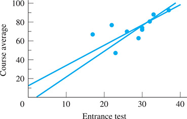
Fig. 22.22
| Student | Entrance Test Score, Based on 40 | Course Average, Based on 100 |
|---|---|---|
| A | 29 | 63 |
| B | 33 | 88 |
| C | 22 | 77 |
| D | 17 | 67 |
| E | 26 | 70 |
| F | 37 | 93 |
| G | 30 | 72 |
| H | 32 | 81 |
| I | 23 | 47 |
| J | 30 | 74 |
Since there are many ways of visually drawing a line through a set of points, we must establish criteria for determing which one fits the best.
There are a number of different methods of determining the straight line that best fits the given data points. We employ the method that is most widely used: the method of least squares. The basic principle of this method is that the sum of the squares of the deviations of all data points from the best line (in accordance with this method) has the least value possible. By deviation, we mean the difference between the y-value of the line and the y-value for the point (of original data) for a particular value of x.
EXAMPLE 2 Deviation and least squares line
In Fig. 22.23, the deviations of some of the points of Example 1 are shown. The point (29, 63) (student A of Example 1) has a deviation of 8 from the indicated line in the figure. Thus, we square the value of this deviation to obtain 64. In order to find the equation of the straight line that best fits the given points, the method of least squares requires that the sum of all such squares be a minimum.
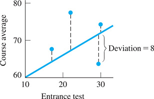
Fig. 22.23
Therefore, in applying this method of least squares, it is necessary to use the equation of a straight line and the coordinates of the points of the data. The deviations of all of these data points are determined, and these values are then squared. It is then necessary to determine the constants for the slope m and the y-intercept b in the equation of a straight line for which the sum of the squared values is a minimum. To do this requires certain methods of advanced mathematics.
Using the methods that are required from advanced mathematics, it can be shown that the equation of the least-squares line
is found by calculating the values of the slope m and the y-intercept b by using the formulas
and
In the above equations, the x’s and y’s are the values of the coordinates of the points in the given data, and n is the number of points of data.
The following examples illustrate finding the least-squares line by use of Eqs. (22.8) and (22.9). Note that much of the work involved is finding the required sums for x, y, xy, and . All of the calculations can be done on a calculator.
EXAMPLE 3 Finding equation of least-squares line—course averages
Find the least-squares line for the data of Example 1.
Here, the x-values will be the entrance-test scores and the y-values are the course averages.
| x | y | xy | |
|---|---|---|---|
| 29 | 63 | 1,827 | 841 |
| 33 | 88 | 2,904 | 1089 |
| 22 | 77 | 1,694 | 484 |
| 17 | 67 | 1,139 | 289 |
| 26 | 70 | 1,820 | 676 |
| 37 | 93 | 3,441 | 1369 |
| 30 | 72 | 2,160 | 900 |
| 32 | 81 | 2,592 | 1024 |
| 23 | 47 | 1,081 | 529 |
| 30 | 74 | 2,220 | 900 |
| 279 | 732 | 20,878 | 8101 |
Thus, the equation of the least-squares line is
The regression feature on a calculator can also be used to find the least-squares line. Figure 22.24(a) shows the regression equation, and Fig. 22.24(b) shows its graph through the scatterplot. Note that the calculator uses a to represent the slope of the regression line instead of m.
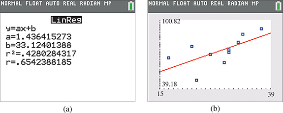
Fig. 22.24
Graphing calculator keystrokes: bit.ly/
The regression line can be used to predict the approximate course average based on the entrance test score. For example, to predict the course average for a student who scored 30 on the entrance test, we substitute 30 for x and evaluate:
If we store the regression line in when doing the regression, then we can predict the course average by entering (30) as shown in Fig. 22.25. Thus, the predicted course average is 76.
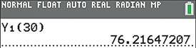
Fig. 22.25
Graphing calculator keystrokes: bit.ly/
NOTE
[In regression, interpolation refers to predictions that are made using values inside the range of the given data and extrapolation refers to predictions made with values outside the range of the given data.]
The prediction made in Example 3 was interpolation since the score of 30 is between the minimum and maximum entrance test scores.
MEASURING THE STRENGTH OF LINEAR CORRELATION: r and r2
Note that the calculator screen in Fig. 22.24(a) shows values of r and in addition to the regression line. These two values measure how well the regression line fits the data. The correlation coefficient r is defined by where and are the standard deviations of the x-values and y-values, respectively, and m is the slope of the regression line. Also, the sign of r is the same as the sign of the slope of the regression line. In Example 3, which indicates a moderate level of positive correlation. The coefficient of determination (the square of r) has an interesting interpretation. In Example 3, which means that 42.8% of the variation in the final course averages can be explained by their linear relationship with entrance-test scores.
NOTE
[Because of its definition, the values of r always lie in the range If r is close to 1 or then there is strong correlation, which means the regression line fits the data points well.]
NOTE
[When viewed as a percentage, it represents the percentage of variation in the y-variable that is explained by the linear model. The value of will always lie between 0% and 100%. The closer it is to 100%, the better the regression line fits the data points.]
NOTE
[To summarize, r-values close to 1 or and close to 100% indicate the regression model fits the data points very well.]
EXAMPLE 4 Least-squares line—drug in bloodstream
In a research project to determine the amount of a drug that remains in the bloodstream after a given dosage, the amounts y (in mg of drug/dL of blood) were recorded after t h, as shown in the table below. Find the least-squares line for these data, expressing y as a function of t. Sketch the graph of the line and data points.
The calculations are as follows:
| t (h) | 1.0 | 2.0 | 4.0 | 8.0 | 10.0 | 12.0 |
| y (mg/dL) | 7.6 | 7.2 | 6.1 | 3.8 | 2.9 | 2.0 |
| t | y | ty | |
|---|---|---|---|
| 1.0 | 7.6 | 7.6 | 1.0 |
| 2.0 | 7.2 | 14.4 | 4.0 |
| 4.0 | 6.1 | 24.4 | 16 |
| 8.0 | 3.8 | 30.4 | 64 |
| 10.0 | 2.9 | 29.0 | 100 |
| 12.0 | 2.0 | 24.0 | 144 |
| 37.0 | 29.6 | 129.8 | 329 |
The equation of the least-squares line is This line is useful in determining the amount of the drug in the bloodstream at any given time. For example, using the regression line, the predicted amount of drug in the bloodstream after 13 hours is 1.4 mg/dL (extrapolation).
The calculator display of the regression line and its graph through the scatterplot are shown in Fig. 22.26(a) and (b), respectively. Note that r is very close to and is close to 1 (or 100%). This indicates a very good fit.
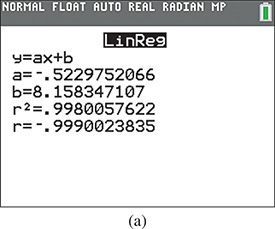
Fig. 22.26
Graphing calculator keystrokes:
bit.ly/
CAUTION
When making predictions, be careful to round only the final estimate, not the values in the regression equation. Small amounts of rounding in the regression equation can lead to fairly large errors in the estimates. When possible, use calculator stored regression equations to make predictions as shown in Example 3.
EXERCISES 22.6
In Exercises 1–14, find the equation of the least-squares line for the given data. Graph the line and data points on the same graph.
x 1 2 3 4 5 y 3 7 9 9 12 x 1 2 3 4 5 6 7 y 10 17 28 37 49 56 72 x 20 26 30 38 48 60 y 160 145 135 120 100 90 x 1 3 6 5 8 10 4 7 3 8 y 15 12 10 8 9 2 11 9 11 7 The speed v (in m/s) of sound was measured as a function of the temperature T (in ) with the following results. Find v as a function of T.
T () 0 10 20 30 40 50 60 v (m/s) 331 337 344 350 356 363 369 In an electrical experiment, the following data were found for the values of current and voltage for a particular element of the circuit. Find the voltage V as a function of the current i. Then predict the voltage if . Is this interpolation or extrapolation?
Current (mA) 15.0 10.8 9.30 3.55 4.60 Voltage (V) 3.00 4.10 5.60 8.00 10.50 A particular muscle was tested for its speed of shortening as a function of the force applied to it. The results appear below. Find the speed as a function of the force. Then predict the speed if the force is 15.0 N. Is this interpolation or extrapolation?
Force (N) 60.0 44.2 37.3 24.2 19.5 Speed (m/s) 1.25 1.67 1.96 2.56 3.05 The altitude h (in m) of a rocket was measured at several positions at a horizontal distance x (in m) from the launch site, shown in the table. Find the least-squares line for h as a function of x.
x (m) 0 500 1000 1500 2000 2500 h (m) 0 1130 2250 3360 4500 5600 In testing an air-conditioning system, the temperature T in a building was measured during the afternoon hours with the results shown in the table. Find the least-squares line for T as a function of the time t from noon. Then predict the temperature when Is this interpolation or extrapolation?
t (h) 0.0 1.0 2.0 3.0 4.0 5.0 T () 20.5 20.6 20.9 21.3 21.7 22.0 The pressure p was measured along an oil pipeline at different distances from a reference point, with results as shown. Find the least-squares line for p as a function of x using a calculator. Then predict the pressure at a distance of . Is this interpolation or extrapolation?
x (ft) 0 100 200 300 400 650 630 605 590 570 The heat loss L per hour through various thicknesses of a particular type of insulation was measured as shown in the table. Find the least-squares line for L as a function of t using a calculator.
t (in.) 3.0 4.0 5.0 6.0 7.0 L (Btu) 5900 4800 3900 3100 2450 In an experiment on the photoelectric effect, the frequency of light being used was measured as well as the stopping potential (the voltage just sufficient to stop the photoelectric effect) with the results given below. Use a calculator to find the least-squares line for V as a function of f. The frequency for is known as the threshold frequency. From the graph determine the threshold frequency.
f (PHz) 0.550 0.605 0.660 0.735 0.805 0.880 V (V) 0.350 0.600 0.850 1.10 1.45 1.80 If gas is cooled under conditions of constant volume, it is noted that the pressure falls nearly proportionally as the temperature. If this were to happen until there was no pressure, the theoretical temperature for this case is referred to as absolute zero. In an elementary experiment, the following data were found for pressure and temperature under constant volume.
T () 0.0 20 40 60 80 100 P(kPa) 133 143 153 162 172 183 Use a calculator to find the least-squares line for P as a function of T, and from the graph determine the value of absolute zero found in this experiment.
In Exercises 15–18, find and interpret the values of r and for the given data.