
22.4 Normal Distributions
Normal Distributions • Empirical Rule • z-Score • Standard Normal Distribution • Applications of Normal Distributions • Sampling Distribution of • Standard Error
The distributions in the previous sections have been for a limited number of values. Let us now consider a very large population, such as the useable lifetime of all the AA batteries sold in the world in a year. It could have a large number of classes with many values within each class.
We would expect a histogram for this very large population to have its maximum frequency very near the mean and taper off to smaller frequencies on either side. It would probably be shaped something like the curve shown in Fig. 22.10.

Fig. 22.10
The smooth bell-shaped curve in Fig. 22.10 shows the normal distribution of a population large enough that the distribution is considered to be continuous. Using advanced methods, its equation is found to be
Here, is the population mean and is the population standard deviation, and and e are the familiar numbers first used in Chapters 2 and 12, respectively.
From Eq. (22.4), we can see that any particular normal distribution depends on the values of and . The horizontal location of the curve depends on and the spread of the curve depends on but the bell shape remains. The next example illustrates the shapes of different normal distributions.
EXAMPLE 1 Different normal distributions
In Fig. 22.11, for the left curve, and whereas for the right curve, and
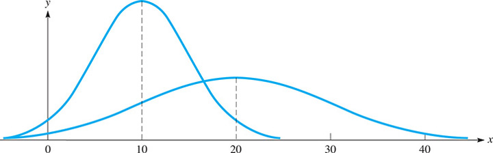
Fig. 22.11
Although there are many possible normal distributions (depending on the mean and standard deviation), the total area under any normal curve is 1 (or 100%). Also, the percentages of the values that are within one, two, or three standard deviations of the mean are the same for all normal distributions. This fact is called the empirical rule and is stated below.
EXAMPLE 2 Empirical rule—achievement test scores
The scores on a certain achievement test are normally distributed with a mean of 500 and a standard deviation of 50. What percentage of the scores are (a) between 400 and 600, and (b) higher than 550?
Since 400 is two standard deviations below the mean and 600 is two standard deviations above the mean, about 95% of all scores are between these values.
The value 550 is one standard deviation above the mean. This means that about 34% (half of 68%) of the scores are between 500 and 550. Therefore, the percentage of scores that are higher than 550 is about
NOTE
[Remember that the total area under any normal curve is . Because a normal curve is symmetric, the area on either side of the mean is .]
In order to find percentages of a normal distribution that lie between fractional increments of the standard deviation, we convert the given values to z-scores (or standard scores) and then use the standard normal distribution. It is calculated using the following formula:
NOTE
[The z-score of a particular value x tells us the number of standard deviations the given value of x is above or below the mean.]
A positive z-score indicates the value is above the mean, whereas a negative z-score indicates it is below the mean.
EXAMPLE 3 z-scores—achievement test results
Using the mean and standard deviation given in Example 2, find and interpret the z-scores of achievement test results of (a) 610 and (b) 435.
The test result of 610 has a z-score of This test result is 2.2 standard deviations above the mean. This is a very high test score, which is rarely obtained.
The test result of 435 has a z-score of This test result is 1.3 standard deviations below the mean. This score is below the mean, but fairly typical.
By converting given values to z-scores, we can use the standard normal distribution to find areas (or percentages). Like any normal curve, the total area under the curve is 1. However, the horizontal axis is labeled with z-scores, which can be interpreted as the number of standard deviations above or below the mean. Figure 22.13 shows the standard normal curve. Note that almost all of the area is between and (99.7% according to the empirical rule). Standard normal tables, such as the one given in Table 22.1 on the next page, can be used to find areas under the standard normal curve.
NOTE
[The standard normal distribution has a mean of 0 and a standard deviation of 1.]
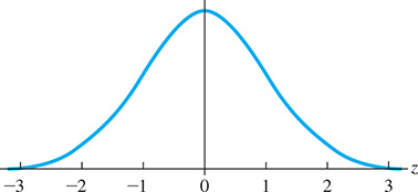
Fig. 22.13
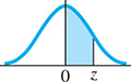
NOTE
[The areas in Table 22.1 represent the area between the mean of 0 and the given z-score.]
Other types of areas can be found by adding or subtracting as needed.
Table 22.1 Standard Normal (z) Distribution
| z | Area | z | Area | z | Area | z | Area | z | Area | z | Area |
|---|---|---|---|---|---|---|---|---|---|---|---|
| 0.1 | 0.0398 | 0.6 | 0.2257 | 1.1 | 0.3643 | 1.6 | 0.4452 | 2.1 | 0.4821 | 2.6 | 0.4953 |
| 0.2 | 0.0793 | 0.7 | 0.2580 | 1.2 | 0.3849 | 1.7 | 0.4554 | 2.2 | 0.4861 | 2.7 | 0.4965 |
| 0.3 | 0.1179 | 0.8 | 0.2881 | 1.3 | 0.4032 | 1.8 | 0.4641 | 2.3 | 0.4893 | 2.8 | 0.4974 |
| 0.4 | 0.1554 | 0.9 | 0.3159 | 1.4 | 0.4192 | 1.9 | 0.4713 | 2.4 | 0.4918 | 2.9 | 0.4981 |
| 0.5 | 0.1915 | 1.0 | 0.3413 | 1.5 | 0.4332 | 2.0 | 0.4772 | 2.5 | 0.4938 | 3.0 | 0.4987 |
EXAMPLE 4 Finding area under the standard normal curve
Find the area under the standard normal curve between and as shown in Fig. 22.14.

Fig. 22.14
Using Table 22.1, the area between and is 0.4918. The area between and is 0.2881. Therefore, the area between and is found by subtracting:
In applications involving normal distributions, areas are found by first converting the values to z-scores and then using the standard normal distribution. This is illustrated in the next example.
EXAMPLE 5 Application of normal distribution—battery lifetimes
The lifetimes of a certain type of watch battery are normally distributed with a mean of 400 days and a standard deviation of 50 days. What percentage of batteries will last (a) between 360 days and 460 days, (b) more than 320 days, and (c) less than 280 days?
We first find the z-score of each value: and We wish to find the area between these two z-scores as shown in Fig. 22.15. Using Table 22.1, the area between and is 0.2881 and the area between and is 0.3849. Thus, the total area is found by adding: This means that 67.3% of the batteries will last between 360 and 460 days.

Fig. 22.15
We begin by finding the z-score of 320 days:
We wish to find the area to the right of shown in Fig. 22.16. The area between and is 0.4452. Since the area to the right of is 0.5, we add to get the total area: This means that 94.52% of the batteries will last longer than 320 days.
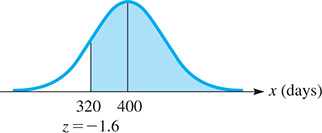
Fig. 22.16
The z-score of 280 is The area to the left of this (see Fig. 22.17) is Therefore, only 0.82% of the batteries will last fewer than 280 days.

Fig. 22.17
Instead of using Table 22.1, a calculator can also be used to find areas under the standard normal curve. The normalcdf feature calculates the area between a specified lower and upper bound. When using z-scores in the normalcdf feature, a 10 can be used as an upper bound for areas that continue indefinitely to the right. This is because there is virtually no area more than 10 standard deviations away from the mean. Similarly, a can be used as a lower bound for areas that continue to the left. Figure 22.18 shows the calculator’s evaluations of the areas in this example.
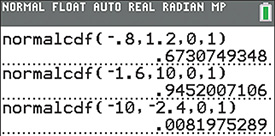
Fig. 22.18
Graphing calculator screenshot: bit.ly/
THE SAMPLING DISTRIBUTION OF x̄
Suppose we selected all possible samples of size n from a population with mean and standard deviation and we calculated the sample mean for each sample. We would have a huge number of sample means. The way in which these sample means are distributed is called the sampling distribution of . The following summarizes three very important facts about this sampling distribution.
By knowing the mean, standard deviation, and shape of the sampling distribution, it is possible to find the likelihood that the mean of a sample falls within certain limits. This is illustrated in the following example.
EXAMPLE 6 Sampling distribution of x̄ —airline passenger weights
The FAA standards assume that adult airline passengers and their carry-on bags have an average weight of 190 lb in the summer. If the standard deviation of these weights is 25 lb, find the likelihood that for a sample of 100 passengers, their mean weight is greater than 195 lb.
Since the sample size is the sampling distribution of is approximately normally distributed with a mean of 190 and a standard deviation of Thus, the z-score of 195 is
We wish to find the area to the right of which is In other words, 2.28% of samples of 100 passengers will have means over 195 lb.
EXERCISES 22.4
In Exercises 1–4, make the given changes in the indicated examples of this section and then solve the indicated problem.
 In Example 1, change the second from 10 to 5 and then describe the curve that would result in terms of either or both curves shown in Fig. 22.11.
In Example 2, what percentage of the test scores are between 350 and 650?
In Example 3, find and interpret the z-score of an achievement test score of 630.
In Example 5(b), change 320 to 360 and then find the resulting percentage of batteries.
In Exercises 5–8, use the following information. If the weights of cement bags are normally distributed with a mean of 60 lb and a standard deviation of 1 lb, use the empirical rule to find the percent of the bags that weigh the following:
Between 58 lb and 62 lb
Between 59 lb and 61 lb
Less than 63 lb
More than 62 lb
In Exercises 9–12, use the following information. A standardized math test has a mean score of 200 and a standard deviation of 15. Find and interpret the z-scores of the following math test scores.
218
179
164
233
In Exercises 13–16, use the following data. It has been previously established that for a certain type of AA battery (when newly produced), the voltages are distributed normally with and .
According to the empirical rule, what percent of the batteries have voltages between 1.45 V and 1.55 V?
What percent of the batteries have voltages between 1.52 V and 1.58 V?
What percent of the batteries have voltages below 1.54 V?
What percent of the batteries have voltages above 1.64 V?
In Exercises 17–24, use the following data. The lifetimes of a certain type of automobile tire have been found to be distributed normally with a mean lifetime of 100,000 km and a standard deviation of 10,000 km. Answer the following questions.
What percent of the tires will last between 85,000 km and 100,000 km?
What percent of the tires will last between 95,000 km and 115,000 km?
In a sample of 5000 of these tires, how many can be expected to last more than 118,000 km?
If the manufacturer guarantees to replace all tires that do not last 75,000 km, what percent of the tires may have to be replaced under this guarantee?
In a sample of 100 of these tires, find the likelihood that the mean lifetime for the sample is less than 98,200.
- What happens to the standard error of the mean as n increases? Use the formula for the standard error to help explain your answer.
What percent of the samples of 100 of these tires should have a mean lifetime of more than 102,000 km?
If 144 of the tires are randomly selected, find the percent chance that the mean lifetime is more than 102,000.
In Exercises 25–30, solve the given problems,
With 75.8% of the area under the normal curve to the right of z, find the z-value.
With 21% of the area under the normal curve between and to the right of find .
With 59% of the area under the normal curve between and to the left of find .
With 5.8% of the area under the normal curve between and to the left of find .
The residents of a city suburb live at a mean distance of 16.0 km from the center of the city, with a standard deviation of 4.0 km. What percent of the residents live between 12.0 km and 18.0 km of the center of the city?
- For the data on the number of Android apps in Exercise 19 of Section 22.1, find the percent of the data that lie within one, two, and three standard deviations of the mean. Compare these percentages with the ones in the empirical rule.
Answer to Practice Exercises
0.5328
99.7%