10.4 Graphs of y = tan x , y = cot x , y = sec x , y = csc x
Graph of • Reciprocal Functions • Asymptotes • Graphs of
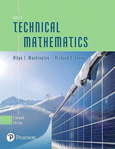
The graph of is displayed in Fig. 10.23. Because from Section 4.3 we know that and we are able to find values of and and graph these functions, as shown in Figs. 10.24–10.26.

Fig. 10.23
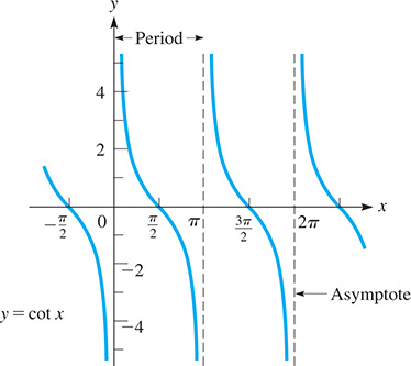
Fig. 10.24
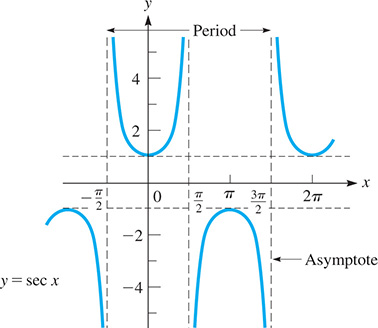
Fig. 10.25

Fig. 10.26
From these graphs, note that the period for and is and that the period of and is The vertical dashed lines are asymptotes (see Sections 3.4 and 21.6). The curves approach these lines, but never actually reach them.
The functions are not defined for the values of x for which the curve has asymptotes. This means that the domains do not include these values of x. Thus, we see that the domains of and include all real numbers, except the values and so on. The domain of and include all real numbers except and so on.
From the graphs, we see that the ranges of and are all real numbers, but that the ranges of and do not include the real numbers between and 1.
To sketch functions such as first sketch and then multiply the y-values by a.
NOTE
[Here, a is not an amplitude, because the ranges of these functions are not limited in the same way they are for the sine and cosine functions.]
Example 1 Sketching graph of y = a sec x
Sketch the graph of
First, we sketch in the curve shown in black in Fig. 10.27. Then we multiply the y-values of this secant function by 2. Although we can only estimate these values and do this approximately, a reasonable graph can be sketched this way. The desired curve is shown in blue in Fig. 10.27.
Fig. 10.27
Using a calculator, we can display the graphs of these functions more easily and more accurately than by sketching them. By knowing the general shape and period of the function, the values for the window settings can be determined.
Example 2 Calculator graph of y = a cot bx
View at least two cycles of the graph of on a calculator.
Because the period of is the period of is Therefore, we choose the window settings as follows:
We must remember to enter the function as because The graphing calculator view is shown in Fig. 10.28. We can view many more cycles of the curve with appropriate window settings.
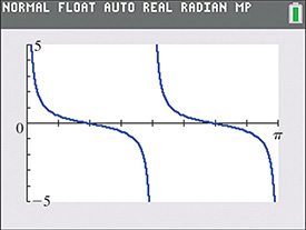
Fig. 10.28
Example 3 Calculator graph of y = a csc(bx + c)
View at least two periods of the graph of on a calculator.
Because the period of csc x is the period of is Recalling that the curve will have the same displacement as Therefore, displacement is There is some flexibility in choosing the window settings, and as an example, we choose the following settings.
With the function is graphed in blue in Fig. 10.29. The graph of is shown in red for reference.
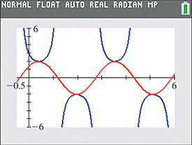
Fig. 10.29
Exercises 10.4
In Exercises 1 and 2, view the graphs on a calculator if the given changes are made in the indicated examples of this section.
In Exercises 3–6, fill in the following table for each function and plot the graph from these points.
| x | 0 | y | ||||||||||||
In Exercises 7–14, sketch the graphs of the given functions by use of the basic curve forms (Figs. 10.23, 10.24, 10.25, and 10.26). See Example 1.
In Exercises 15–24, view at least two cycles of the graphs of the given functions on a calculator.
In Exercises 25–28, solve the given problems. In Exercises 29–32, sketch the appropriate graphs, and check each on a calculator.
 Using the graph of explain what happens to tan x as x gets closer to (a) from the left and (b) from the right.
- Using a calculator, graph and in the same window. When sin x reaches a maximum or minimum, explain what happens to csc x.
Write the equation of a secant function with zero displacement, a period of and that passes through
Use a graphing calculator to show that for although sin x and tan x are nearly equal for the values near zero.
Near Antarctica, an iceberg with a vertical face 200 m high is seen from a small boat. At a distance x from the iceberg, the angle of elevation of the top of the iceberg can be found from the equation Sketch x as a function of
In a laser experiment, two mirrors move horizontally in equal and opposite distances from point A. The laser path from and to point B is shown in Fig. 10.30. From the figure, we see that Sketch the graph of for
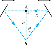
Fig. 10.30
A mechanism with two springs is shown in Fig. 10.31, where point A is restricted to move horizontally. From the law of sines, we see that Sketch the graph of b as a function of A for and
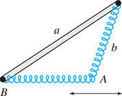
Fig. 10.31
A cantilever column of length L will buckle if too large a downward force P is applied d units off center. The horizontal deflection x (see Fig. 10.32) is where k is a constant depending on P, and For a constant d, sketch the graph of x as a function of kL.
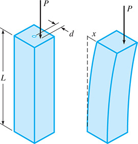
Fig. 10.32